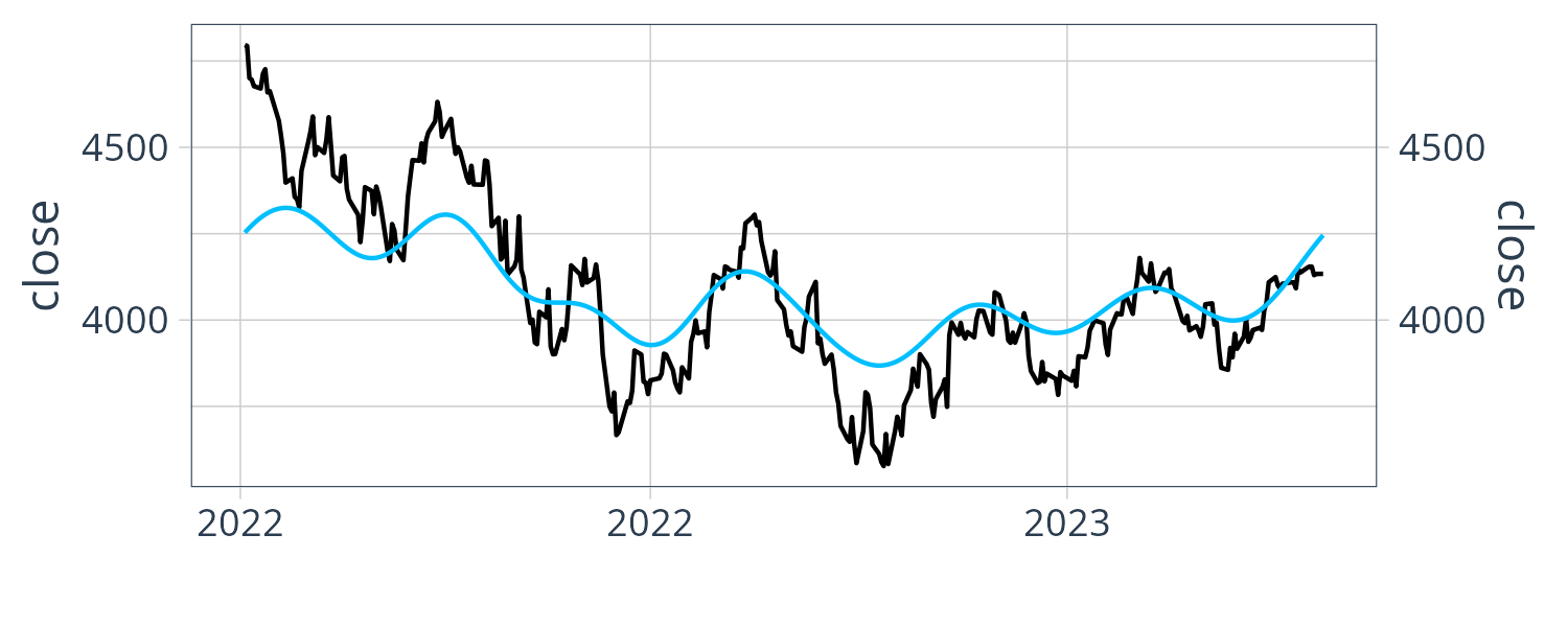
Complex exponential signals appear a lot in Digital Signal Processing and in this article, we are going to explore the basic tenets and intuitive understanding of what exactly they are and how they are related to real signals.

\[\begin{aligned} e^{i\times 0} &= \mathrm{cos}(0) + i \mathrm{sin}(0)\\ &= 1 + 0\\ &= 1\\[5pt] e^{i\frac{\pi}{2}} &= \mathrm{cos}(\frac{\pi}{2}) + i \mathrm{sin}(\frac{\pi}{2})\\ &= 0 + i \times 1\\ &= i\\[5pt] e^{i\pi} &= \mathrm{cos}(\pi) + i \mathrm{sin}(\pi)\\ &= -1 + 0\\ &= -1\\[5pt] e^{i\frac{3\pi}{2}} &= \mathrm{cos}(\frac{3\pi}{2}) + i \mathrm{sin}(\frac{3\pi}{2})\\ &= 0 + i \times -1\\ &= -i \end{aligned}\]

Other points can be computed by their inputing the relevant angles.

When you introduce \(t\) such that:

\[\begin{aligned} e^{i\omega t} \end{aligned}\]

Now the value will vary with time. \(\omega\) is the angular velocity in radians/sec.

So for \(t = 0\) to \(t = 1\), the point will move from \(+1\) to \(\omega\) radians.

For example:

\[\begin{aligned} \omega &= 2\pi\\ e^{i\omega \times 0} &= 1\\ e^{i\omega \times 1} &= e^{i\omega}\\ &= e^{i 2 \pi}\\ &= 1 \end{aligned}\]

So in the above example, it will complete one revolution per second. If \(\omega = \pi\), it will complete half a revolution per second.

Introduction to Sinusoidal Signals

Let us start with a simple sine wave. Below is the R code to generate a 3-period \(T = 2\pi\) sine wave:

library(fpp3)
library(tidyquant)

num_periods <- 3
f <- 1
t <- seq(0, f * num_periods, 0.01)   
signal <- tsibble(
  t = t,
  y = sin(2 * pi * f * t),
  index = t
)

signal |>
  autoplot(y) +
  xlab("t") +
  theme_tq()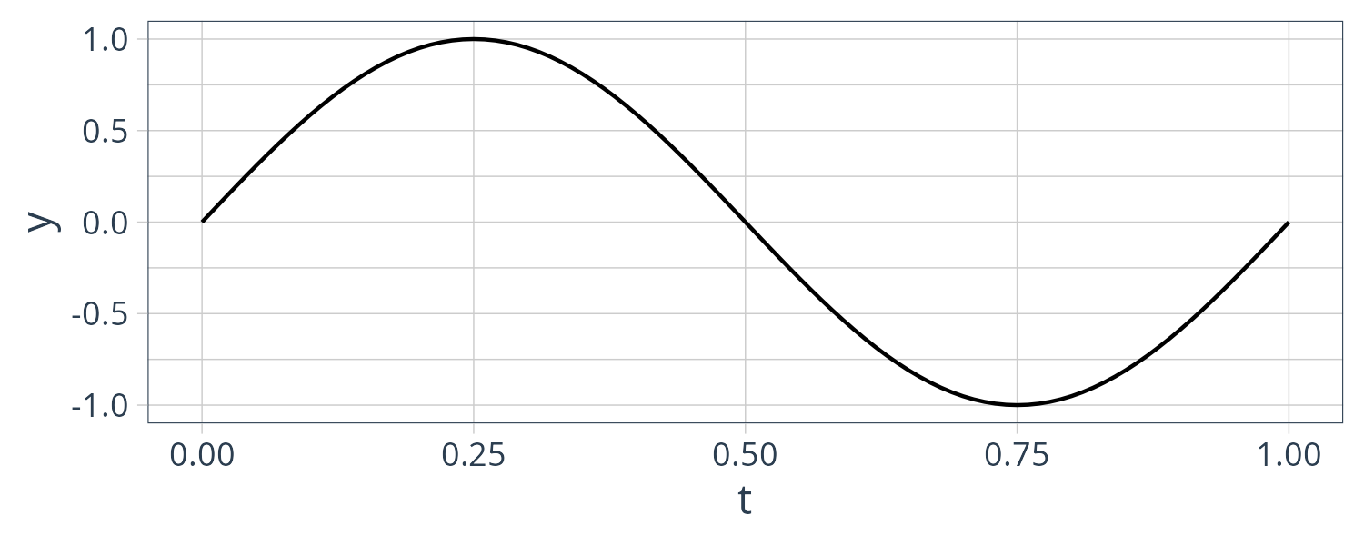

A sine wave can be represented by the following complex exponential:

\[\begin{aligned} y(t) &= \mathrm{sin}(t)\\ &= \frac{1}{2} \Big[(\mathrm{cos}\ t + i\ \mathrm{sin}\ t) - (\mathrm{cos}\ t - i\ \mathrm{sin}\ t)\Big]\\ &= \frac{e^{it} - e^{-it}}{2} \end{aligned}\]

Euler’s formula states that:

\[\begin{aligned} e^{it} &= \mathrm{cos}\ t + i\ \mathrm{sin}\ t \end{aligned}\]

One can derive the Euler’s formula from the Taylor Series representation of sine and cosine waves:

\[\begin{aligned} \mathrm{cos}\ t &= 1 - \frac{t^{2}}{2!} + \frac{t^{4}}{4!} - \frac{t^{6}}{6!} + \cdots\\[5pt] \mathrm{sin}(it) &= it - \frac{(it)^{3}}{3!} + \frac{(it)^{5}}{5!} - \frac{(it)^{7}}{7!} + \cdots\\[5pt] e^{it} &= 1 + it + \frac{(it)^{2}}{2!} + \frac{(it)^{3}}{3!} + \frac{(it)^{4}}{4!} + \cdots\\ &= 1 + it - \frac{t^{2}}{2!} - \frac{it^{3}}{3!} + \frac{t^{4}}{4!} - \frac{it^{5}}{5!} - \cdots\\ &= 1 - \frac{t^{2}}{2!} + \frac{t^{4}}{4!} - \cdots + it - \frac{it^{5}}{5!} + \cdots\\ &= \mathrm{cos}\ t + i\ \mathrm{sin}\ t \end{aligned}\]

Similarly for cosine:

\[\begin{aligned} y(t) &= \mathrm{cos}(t)\\ &= \frac{1}{2} \Big[(\mathrm{cos}\ t + i\ \mathrm{sin}\ t) + (\mathrm{cos}\ t - i\ \mathrm{sin}\ t)\Big]\\ &= \frac{e^{it} + e^{-it}}{2} \end{aligned}\]

We can verify this in R:

t <- seq(0, f * num_periods, 0.01)
y <- (exp(1i * t) - exp(-1i * t)) / 2    

signal <- tsibble(
  t = t,
  y = sin(2 * pi * f * t),
  index = t
)

signal |>
  autoplot(y) +
  xlab("t") +
  theme_tq()

Which should reproduce the same sine graph as above.

To generalize further, we add the concept of frequency into the equations. Frequency is the number of cycles per time unit. It will be easier if we think in terms of number of radians per time unit (radian frequency).

\[\begin{aligned} \omega &= 2\pi f \end{aligned}\]

Previously, we assume the frequency is 1 cycle per time unit. Given \(f = 1\):

\[\begin{aligned} f &= 1\\[5pt] \omega &= 2\pi\\[5pt] \mathrm{sin}(\omega t) &= \mathrm{sin}(2\pi f t) \end{aligned}\]

If we double the frequency to \(f = 2\), we get the following equation and graph:

\[\begin{aligned} \omega &= 2\pi * 2\\[5pt] \mathrm{sin}(\omega\ t) &= \mathrm{sin}(4\pi t) \end{aligned}\]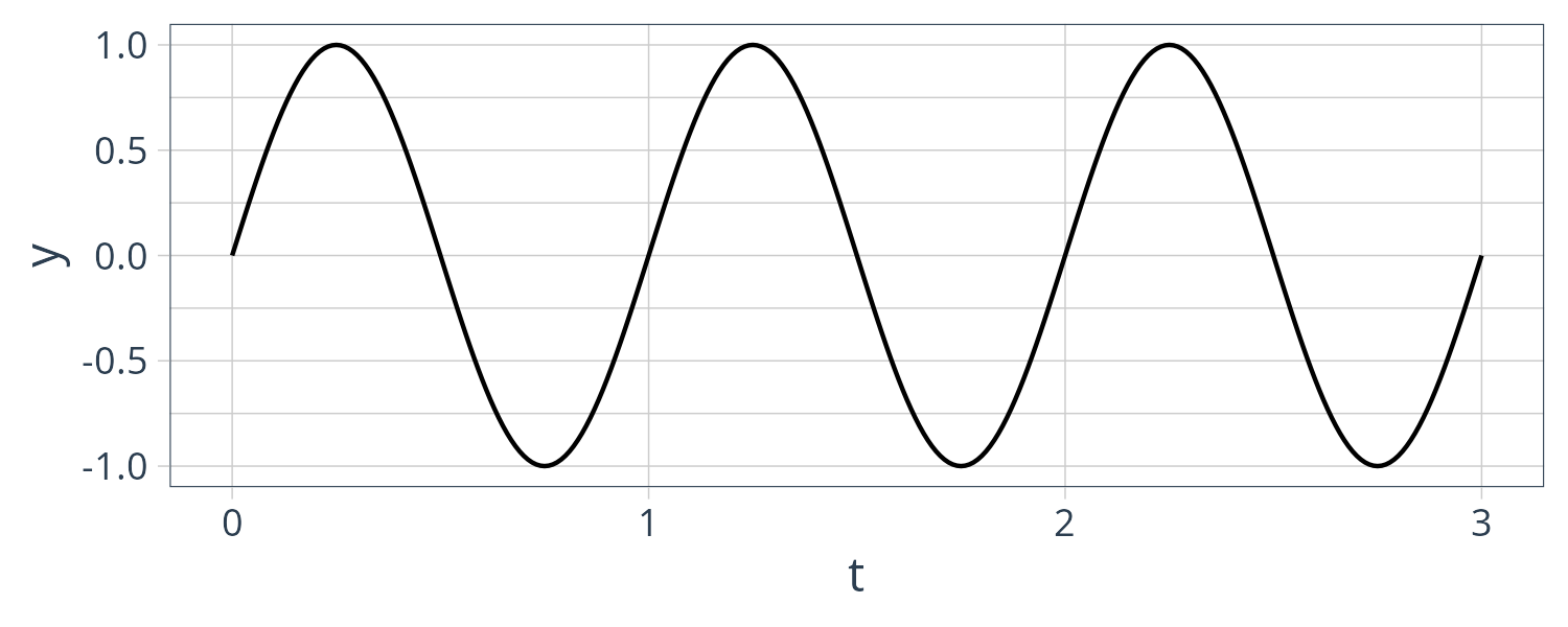

We can derive any signals we want by mixing a particular mixture of sine and cosine waves. To make the example more interesting, let us find a mixture of signals to fit the closing price of SP500. Taking the closing price of SPY from 2020 to Apr of 2023, we try to fit a sinusoidal signal using only 10 distinct complex coefficients.

coefs <- c(
  1945270.375 + 0.000i,
  50368.755 - 38436.030i,
  9238.201 - 20881.416i,
  -14268.049 - 17675.716i,    
  18343.644 + 9461.970i,
  1564.889 - 23749.279i,
  21452.220 - 6398.907i,
  -225.060 - 8115.913i,
  -8442.376 + 2129.005i,
  1882.040 + 2207.576i
)

And using the following Fourier series:

\[\begin{aligned} y[n] &= \frac{1}{N}\sum_{k = 0}^{(10 - 1)}C_{k}e^{ik\frac{2\pi}{N}n} \end{aligned}\]

We are able to get the following graph:

Phase Shift

It is possible to rewrite a phase shifted signal into a combination of sine and cosine terms with the same frequency.

\[\begin{aligned} c_{k} \mathrm{cos}(\omega_{k}t - \phi_{k}) &= a_{k} \mathrm{cos}(\omega_{k}t) + b_{k} \mathrm{sin}(\omega_{k}t)\\[5pt] c_{k} \mathrm{cos}(\omega_{k}t + \phi_{k}) &= a_{k} \mathrm{cos}(\omega_{k}t) - b_{k} \mathrm{sin}(\omega_{k}t)\\[5pt] c_{k} \mathrm{sin}(\omega_{k}t - \phi_{k}) &= a_{k} \mathrm{cos}(\omega_{k}t) - b_{k} \mathrm{sin}(\omega_{k}t)\\[5pt] c_{k} \mathrm{sin}(\omega_{k}t + \phi_{k}) &= a_{k} \mathrm{cos}(\omega_{k}t) + b_{k} \mathrm{sin}(\omega_{k}t)\\[5pt] c_{k} &= \sqrt{a_{k}^{2} + b_{k}^{2}}\\[5pt] \phi_{k} &= \mathrm{tan}^{-1}\Big(\frac{a_{k}}{b_{k}}\Big) \end{aligned}\]

This can be derived by this using the following trigonometric identities:

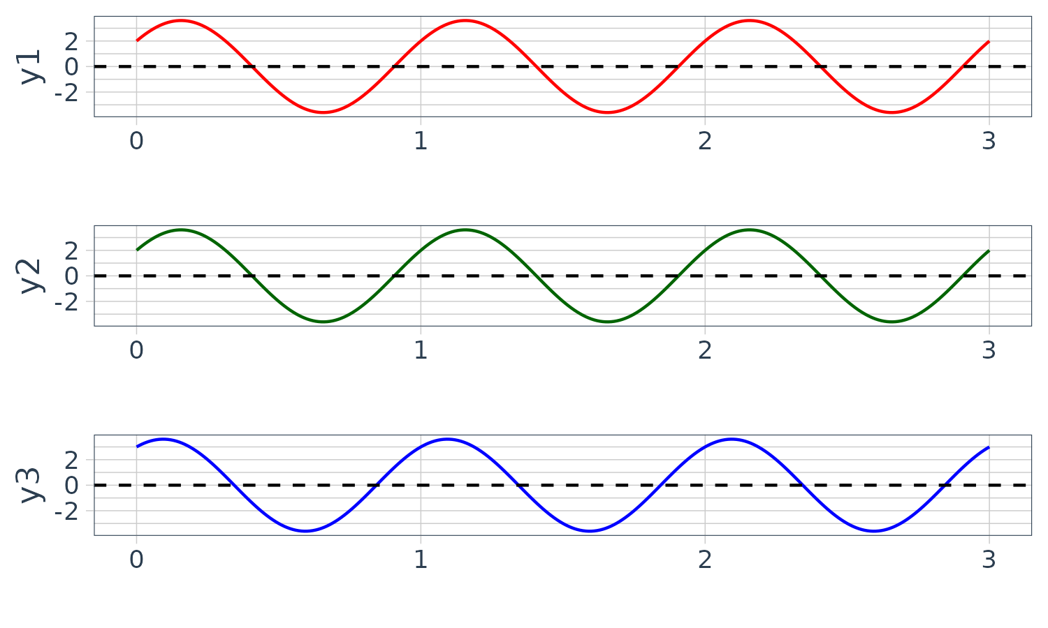
\[\begin{aligned} \mathrm{cos}(\theta \pm \phi) &= \mathrm{cos}\ \theta \ \mathrm{cos}\ \phi \mp \mathrm{cos}\ \theta \ \mathrm{cos}\ \phi\\[5pt] \mathrm{sin}(\theta \pm \phi) &= \mathrm{sin}\ \theta \ \mathrm{cos}\ \phi \pm \mathrm{cos}\ \theta \ \mathrm{sin}\ \phi\\[5pt] a &= c\ \mathrm{sin}(\phi)\\[5pt] b &= c\ \mathrm{cos}(\phi)\\[5pt] a^{2} + b^{2} &= c^{2}\ \mathrm{sin}^{2}(\phi) + c^{2}\ \mathrm{cos}^{2}(\phi)\\[5pt] \frac{a}{b} &= \frac{c\ \mathrm{sin}(\phi)}{c\ \mathrm{cos}(\phi)}\\ &= \mathrm{tan}(\phi)\\[5pt] \phi &= \mathrm{tan}^{-1}\Big(\frac{a}{b}\Big) \end{aligned}\]

We now plot the same wave represented in the following 3 forms. A combination of sine and cosine waves, a phase shifted cosine wave, and a phase shifted sine wave. Note that they all give the same waveform:

num_periods <- 3
a <- 2
b <- 3
c <- sqrt(a^2 + b^2)
phi <- atan(a / b)
omega <- 2 * pi * f
f <- 1
t <- seq(0, f * num_periods, 0.01)

signal <- tsibble(
  t = t,
  y1 = a * cos(omega * t) + b * sin(omega* t),
  y2 = c * sin(omega * t + phi),
  y3 = c * cos(omega * t - phi),
  index = t
)

plot_grid(
  signal |>
    autoplot(y1, col = "red") +
    geom_hline(yintercept = 0, linetype = "dashed") +     
    theme_tq(),
  signal |>
    autoplot(y2, col = "darkgreen") +
    geom_hline(yintercept = 0, linetype = "dashed") +
    theme_tq(),
  signal |>
    autoplot(y3, col = "blue") +
    geom_hline(yintercept = 0, linetype = "dashed") +
    theme_tq(),
  ncol = 1
)

Phasor and Complex-Valued Time Function

It is also possible to see the phase shift by looking at its corresponding complex exponential representation. Let us also add the amplitude in the equation as well.

\[\begin{aligned} A\mathrm{cos}(\omega t + \phi) &= A\frac{e^{i(\omega t + \phi)} + e^{-i(\omega t + \phi)}}{2}\\ &= A\frac{e^{i\phi}e^{i\omega t} + e^{-i\phi}e^{-i\omega t}}{2}\\ &= \frac{Ae^{i\phi}}{2}e^{i\omega t} + \frac{Ae^{-i\phi}}{2}e^{-i\omega t}\\ A\mathrm{cos}(\omega t - \phi) &= \frac{Ae^{-i\phi}}{2}e^{i\omega t} + \frac{Ae^{i\phi}}{2}e^{-i\omega t} \end{aligned}\]

Similarly for sine function (note the \(i\) in the denominator):

\[\begin{aligned} A\mathrm{sin}(\omega t + \phi) &= \frac{Ae^{i\phi}}{2i}e^{i\omega t} - \frac{Ae^{-i\phi}}{2i}e^{-i\omega t}\\ A\mathrm{sin}(\omega t - \phi) &= \frac{Ae^{-i\phi}}{2i}e^{i\omega t} - \frac{Ae^{i\phi}}{2i}e^{-i\omega t} \end{aligned}\]

\(Ae^{i \phi}\) is known as the “phasor” and \(e^{i\omega t}\) the “complex-valued” time function. The phasor can be seen as the starting vector on the 2D complex and the complex-value time function as rotating the starting vector over time. Since \(\|e^{i\omega t}\| = 1\), no scaling is involved and only rotation. The vector will rotate counterclockwise on positive frequency \(\omega > 0\) and clockwise on negative frequency \(-\omega < 0\).

In other words, we can picture for the above phase shifted cosine wave, half of the phasor \(Ae^{i \phi}\) is rotated counterclockwise by \(e^{i\omega t}\) and another half of the reflected phasor \(Ae^{-i \phi}\) is rotated clockwise by \(e^{-i\omega t}\) (complex conjugate) at the radian frequency \(\omega\) per time step \(t\). And after adding the two vectors together, we will always result in a real number for each time step. This is because the vectors are a reflection on the x-axis (real axis), and the imaginary part will cancel out.

This can be demonstrated by the following example. We will explore a cosine wave shifted by \(\frac{\pi}{2}\) which results in a cosine wave reflected on the x-axis.

phi <- pi
phasor1 <- A / 2 * exp(1i * phi)
phasor2 <- A / 2 * exp(-1i * phi)
t <- seq(0, f * 2, 0.01)
dat <- tibble(
  y1 = phasor1 * exp(1i * omega * t),
  y2 = phasor2 * exp(-1i * omega * t)
)
dat |>
  ggplot(aes(x = t, y = Re(y1 + y2))) +    
  geom_line() +
  theme_tq()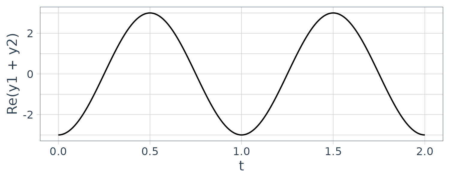

Next, we investigate the 2D complex plot. The vectors are added and projected on the x-axis resuling on a real number. Time is moved in the red, blue, green sequence and we are moving a quarter cycle from t = 0 to t = 0.5 in an interval of 0.125 and amplitude moving from -3 to 3.

phasor1 = A / 2 * exp(1i * phi)
phasor2 <- A / 2 * exp(-1i * phi)
t = seq(0, 0.5, by = 0.125)
dat <- tibble(
  y1 = phasor1 * exp(1i * omega * t),
  y2 = phasor2 * exp(-1i * omega * t)
)
cols <- c("red", "blue", "darkgreen", "red", "blue")      
dat |>
  ggplot() +
  geom_segment(
    aes(
      x = 0, y = 0,
      xend = Re(y1),
      yend = Im(y1)
    ),
    col = cols,
    arrow = arrow(length = unit(0.5, "cm"))
  ) +
  geom_segment(
    aes(
      x = 0, y = 0,
      xend = Re(y2),
      yend = Im(y2)
    ),
    col = cols,
    arrow = arrow(length = unit(0.5, "cm"))
  ) +
  geom_segment(
    aes(
      x = 0, y = 0,
      xend = Re(y1 + y2),
      yend = Im(y1 + y2)
    ),
    col = cols,
    arrow = arrow(length = unit(0.5, "cm"))
  ) +
  scale_x_continuous(
    breaks = seq(-3, 3, by = 1),
    limits = c(-3, 3)
  ) +
  scale_y_continuous(
    breaks = seq(-3, 3, by = 1),
    limits = c(-1.5, 1.5)
  ) +
  theme_tq()

So the way how I would picture a real signal is represented in the complex world, is by splitting each harmonic frequency into two halves. One is a complex conjugate of the other. The imaginary part is always reflected in x-axis (complex conjugate) and hence will cancel out. The imaginary part is important because we need to be able to rotate the vector and represent the phase as an angle in the 2D complex plane.

As for sine wave, we have to divide by \(i\) in the denominator in order to cancel out the imaginary part. The same rotation is carried out but in the imaginary plane and the real part is cancelled out. The final result is divided by \(i\) to make the sine part real.

Adding Sinusoidal Signals

When adding signals with the same frequency but different phase and amplitude, we can always represent the combined wave as a phase shifted cosine (or sine) wave. This can be easiy seen when represented in complex exponential form:

\[\begin{aligned} \sum_{k = 1}^{N}A_{k}\mathrm{cos}(\omega t + \phi_{k}) &= A_{k}e^{i(\omega t + \phi_{k})}\\ &= \sum_{k = 1}^{N}A_{k}e^{i\phi_{k}}e^{i\omega t}\\ &= \Big(\sum_{k = 1}^{N}A_{k}e^{i\phi_{k}}\Big)e^{i\omega t}\\ &= A e^{i\phi} e^{i\omega t}\\ &= A e^{i(\omega t + \phi)}\\ &= A\mathrm{cos}(\omega t + \phi) \end{aligned}\]

Where we define:

\[\begin{aligned} \sum_{k = 1}^{N}A_{k} &= A\\ \sum_{k = 1}^{N}e^{i\phi_{k}} &= e^{i \phi} \end{aligned}\]

So effectively, we aggregate the same frequency terms together and we are left over with waves with distinctive frequency. Each of these distinctive wave will have corresponding conjugate phasors that are rotated by \(e^{\pm i\omega t}\) in their own respective frequency \(\omega\). We will then add them all up at each \(t\) to get the aggregate real value.

Adding each distinctive frequency can also be represented by its individual cosine and sine terms. In the “Phase Shift” section, we showed how each phase shifted signal can be decomposed into its cosine and sine signal. Each cosine and sine components can then be individually added.

\[\begin{aligned} \sum_{k = 1}^{N}A_{k}\mathrm{cos}(\omega t + \phi_{k}) &= \sum_{k = 1}^{N}a_{k}\mathrm{cos}(\omega_{k}t) - \sum_{k = 1}^{N}b_{k}\mathrm{sin}(\omega_{k}t)\\ &= \Big(\sum_{k = 1}^{N}a_{k}\Big)\mathrm{cos}(\omega_{k}t) - \Big(\sum_{k = 1}^{N}b_{k}\Big)\mathrm{sin}(\omega_{k}t)\\ &= a\mathrm{cos}(\omega_{k}t) - b\mathrm{sin}(\omega_{k}t)\\ &= A\mathrm{cos}(\omega t + \phi) \end{aligned}\] \[\begin{aligned} a &= \sum_{k = 1}^{N}a_{k}\\[5pt] b &= \sum_{k = 1}^{N}b_{k}\\[5pt] A &= \sqrt{a^{2} + b^{2}}\\[5pt] \phi &= \mathrm{tan}^{-1}\Big(\frac{a}{b}\Big) \end{aligned}\]

Both the complex exponential form and the sine/cosine form can be used to reprsent signals in different ways. Note the two terms below represent different components and not directly related.

\[\begin{aligned} e^{i(\omega t + \phi_{k})} &= \mathrm{cos}(\omega t + \phi_{k}) + i\mathrm{sin}(\omega t + \phi_{k})\\ &\neq a_{k}\mathrm{cos}(\omega t) - b_{k}\mathrm{sin}(\omega t)\\ \end{aligned}\]

So why do we complicate life by having representing them in different forms? In the future when we cover Fourier series and Fourier transform, we can see how complex exponential simplify the math a lot.

References

The Intuitive Guide to Fourier Analysis and Spectral Estimation: with Matlab Basic Signal Concepts Lecture 3 Complex Exponential Signals

Complex Exponential Signals

Contents:

Complex Exponentials

Introduction to Sinusoidal Signals

Phase Shift

Phasor and Complex-Valued Time Function

Adding Sinusoidal Signals

References

Jason