Fourier Series
Read Post
In this post we will break down a signal into its frequency components and represent it in Fourier Series.
Contents:
Discrete Fourier Series Representation
In discrete time signals, time \(t\) is replaced by the sample number \(n\), and likewise frequency is defined as radians per sample rather than radians per time unit (sec).
\[\begin{aligned} x(t) &= \mathrm{sin}(2\pi f_{0} t)\\ x[n] &= \mathrm{sin}(2\pi f_{0} nT_{s})\\ &= sin\Big( 2\pi\frac{f_{0}}{F_{s}}n\Big) \end{aligned}\]The digital frequency is defined as:
\[\begin{aligned} \Omega &= \frac{2\pi f_{0}}{F_{s}} \end{aligned}\]In contrast with:
\[\begin{aligned} \omega &= 2\pi f_{0} \end{aligned}\]In summary:
\[\begin{aligned} x(t) &= \mathrm{sin}(\omega t)\\ x[n] &= \mathrm{sin}(\Omega n) \end{aligned}\]Fourier Series
A Fourier series consists of weighted harmonics that can represent any periodic wave. A harmonic is a wave of a certain frequency. It can be represented by a sum of cosine and sine harmonics:
\[\begin{aligned} f(t) &= a_{0} + \sum_{k = 1}^{K}a_{k}\mathrm{cos}(2\pi k f_{0}t) + \sum_{k = 1}^{K}b_{k}\mathrm{sin}(2\pi k f_{0}t) \end{aligned}\]\(f_{0}\) is the fundamental frequency (lowest frequency). \(K\) represent the highest frequency and can in fact go into infinity. But this number is capped by the sampling frequency as we will demonstrate later during the Nyquist section. \(a_{0}\) is the constant offset and represent the mean of the series if it is not zero.
Because a sum of cosine and sine waves can be represented by just a cosine wave with a phase shift, the above equation can be simplified to:
\[\begin{aligned} f(t) &= a_{0} + \sum_{k = 1}^{K}c_{k}\mathrm{cos}(2\pi k f_{0}t + \phi)\\ &= a_{0} + \sum_{k = 1}^{K}C_{k}\mathrm{cos}(2\pi f_{k}t + \phi)\\ &= a_{0} + \sum_{k = 1}^{K}C_{k}\mathrm{cos}(\omega_{k}t + \phi) \end{aligned}\]Where:
\[\begin{aligned} f_{k} &= f_{0}k\\ \omega_{k} & = 2\pi f_{k} \end{aligned}\]And finally in complex exponential form. Note k goes from \(-\infty\) to \(\infty\)
\[\begin{aligned} f(t) &= \sum_{k = -\infty}^{\infty}C_{k}e^{i 2\pi \frac{k}{T_{0}}t} \end{aligned}\]Computing \(a_{0}\) coefficient
By taking the integral of \(f(t)\) over the fundamental period \(T_{0}\), we can eliminate the cosine and sine harmonic components. This is because the period of the harmonics are integer multiples of the harmonic period and hence the full cycles would be completed and the area would sum up to 0:
\[\begin{aligned} \int_{0}^{T_{0}} f(t)\ dt &= \int_{0}^{T_{0}} a_{0}\ dt + \int_{0}^{T_{0}} \sum_{k = 1}^{\infty}a_{k}\mathrm{cos}(\omega_{0}kt)\ dt + \int_{0}^{T_{0}}\sum_{k = 1}^{\infty}b_{k}\mathrm{sin}(\omega_{0}kt)\ dt\\ &= \int_{0}^{T_{0}} a_{0}\ dt + \sum_{k = 1}^{\infty}\int_{0}^{T_{0}}a_{k}\mathrm{cos}(\omega_{0}kt)\ dt + \sum_{k = 1}^{\infty}\int_{0}^{T_{0}}b_{k}\mathrm{sin}(\omega_{0}kt)\ dt\\ &= \int_{0}^{T_{0}} a_{0}\ dt + \sum_{k = 1}^{\infty}0 + \sum_{k = 1}^{\infty}0\\ &= \int_{0}^{T_{0}} a_{0}\ dt\\ &= a_{0}T_{0}\\ a_{0} &= \frac{1}{T_{0}}\int_{0}^{T_{0}}f(t)\ dt \end{aligned}\]Computing \(a_{k}\) coefficient
By using trigonometic identities and integrating, we can see that:
\[\begin{aligned} \int_{0}^{T_{0}} \mathrm{cos}(\omega_{0}kt) \mathrm{cos}(\omega_{0}kt)\ dt &= \frac{T_{0}}{2}\\ \int_{0}^{T_{0}} \mathrm{cos}(\omega_{0}mt) \mathrm{cos}(\omega_{0}kt)\ dt &\overset{m \ne k}{=} 0\\ \int_{0}^{T_{0}} \mathrm{cos}(\omega_{0}mt) \mathrm{sin}(\omega_{0}kt)\ dt &= 0 \end{aligned}\]Hence:
\[\begin{aligned} \int_{0}^{T_{0}} a_{k}\mathrm{cos}(\omega_{0}kt) \mathrm{cos}(\omega_{0}kt)\ dt &= a_{k}\frac{T_{0}}{2} \end{aligned}\] \[\begin{aligned} \int_{0}^{T_{0}} f(t)\mathrm{cos}(\omega_{0}kt) \ dt &= a_{k}\frac{T_{0}}{2}\\ a_{k} &= \frac{2}{T_{0}}\int_{0}^{T_{0}} f(t)\mathrm{cos}(\omega_{0}kt) \ dt \end{aligned}\]Computing \(b_{k}\) coefficient
Similar to computing \(a_{k}\):
\[\begin{aligned} \int_{0}^{T_{0}} f(t)\mathrm{sin}(\omega_{0}kt) \ dt &= b_{k}\frac{T_{0}}{2}\\ b_{k} &= \frac{2}{T_{0}}\int_{0}^{T_{0}} f(t)\mathrm{sin}(\omega_{0}kt) \ dt \end{aligned}\]Because all of the integrals except the same harmonics are zeros, it makes it easy to find \(a_{k}\) and \(b_{k}\).
Complex Exponentials
It is also possible to use the complex exponentials representation:
\[\begin{aligned} f(t) &= \sum_{k = -\infty}^{\infty}C_{k}e^{i 2\pi \frac{k}{T_{0}}t} \end{aligned}\]Similar to the trigonometric form, the basis set of complex exponentials are orthogonal to each other:
\[\begin{aligned} \int_{0}^{T_{0}}\mathrm{cos}(i\omega_{0}kt)\mathrm{cos}(i\omega_{0}mt) &\overset{m \ne k}{=} 0\\ \int_{0}^{T_{0}}\mathrm{sin}(i\omega_{0}kt)\mathrm{sin}(i\omega_{0}mt) &\overset{m \ne k}{=} 0\\ \int_{0}^{T_{0}}\mathrm{cos}(i\omega_{0}kt)\mathrm{sin}(i\omega_{0}mt) &\overset{\forall m, k}{=} 0\\ \int_{0}^{T_{0}}e^{i\omega_{0}kt}e^{i\omega_{0}mt}\ dt &\overset{m \ne k}{=} 0 \end{aligned}\]Substituting complex exponentials for trigonometric functions:
\[\begin{aligned} f(t) &= a_{0} + \sum_{k = 1}^{K}a_{k}\mathrm{cos}(\omega_{0}kt) + \sum_{k = 1}^{K}b_{k}\mathrm{sin}(\omega_{0}kt) \\ &= a_{0} + \sum_{k = 1}^{K}\frac{a_{k}}{2}(e^{i\omega kt} + e^{-i \omega kt}) + \sum_{k = 1}^{K}\frac{b_{k}}{2i}(e^{i\omega kt} - e^{-i \omega kt}) \\ &= a_{0} + \sum_{k = 1}^{K}\frac{1}{2}(a_{k} - i b_{k})e^{i\omega_{0}kt} + \sum_{k = 1}^{K}\frac{1}{2}(a_{k} + i b_{k})e^{-i\omega_{0}kt}\\ &= a_{0} + \sum_{k = 1}^{K}A_{k}e^{i\omega_{0}kt} + \sum_{k = 1}^{K}\frac{1}{2}B_{k}e^{-i\omega_{0}kt} \end{aligned}\]Given:
\[\begin{aligned} A_{k} &= \frac{1}{2}(a_{k} - i b_{k})\\ B_{k} &= \frac{1}{2}(a_{k} + i b_{k}) \end{aligned}\]Remember the earlier derivation of \(a_{k}\) and \(b_{k}\):
\[\begin{aligned} a_{k} &= \frac{2}{T_{0}}\int_{0}^{T_{0}} f(t)\mathrm{cos}(\omega_{0}kt) \ dt\\ &= \frac{2}{T_{0}}\int_{0}^{T_{0}} f(t)\frac{1}{2}(e^{i\omega kt} + e^{-i \omega kt}) \ dt\\ b_{k} &= \frac{2}{T_{0}}\int_{0}^{T_{0}} f(t)\mathrm{sin}(\omega_{0}kt) \ dt\\ &= \frac{2}{T_{0}}\int_{0}^{T_{0}} f(t)\frac{1}{2i}(e^{i\omega kt} - e^{-i \omega kt}) \ dt\\ \end{aligned}\]Using the above we can derive the formula for \(A_{k}\):
\[\begin{aligned} A_{k} &= \frac{1}{2}(a_{k} - ib_{k})\\ &= \frac{1}{2}\Big( \frac{2}{T_{0}}\int_{0}^{T_{0}} f(t)\frac{1}{2}(e^{i\omega_{0} kt} + e^{-i \omega_{0} kt}) \ dt - \frac{2}{T_{0}}\int_{0}^{T_{0}} f(t)\frac{1}{2i}(e^{i\omega_{0} kt} - e^{-i \omega_{0} kt}) \ dt \Big)\\ &= \frac{1}{2T_{0}}\Big( \int_{0}^{T_{0}} f(t)e^{i\omega_{0} kt} \ dt + \int_{0}^{T_{0}}f(t)e^{-i \omega_{0} kt} \ dt - \int_{0}^{T_{0}} f(t)e^{i\omega_{0} kt} \ dt + \int_{0}^{T_{0}}f(t)e^{-i \omega_{0} kt} \ dt \Big)\\ &= \frac{1}{T_{0}}\int_{0}^{T_{0}}f(t)e^{i\omega_{0} kt} \ dt \end{aligned}\]We can do the same for \(B_{k}\) as well:
\[\begin{aligned} B_{k} &= \frac{1}{T_{0}}\int_{0}^{T_{0}}f(t)e^{-i\omega_{0} kt} \ dt \end{aligned}\]In summary:
\[\begin{aligned} a_{k} &= \frac{2}{T_{0}}\int_{0}^{T_{0}} f(t)\mathrm{cos}(\omega_{0}kt) \ dt\\ b_{k} &= \frac{2}{T_{0}}\int_{0}^{T_{0}} f(t)\mathrm{sin}(\omega_{0}kt) \ dt\\ A_{k} &= \frac{1}{T_{0}}\int_{0}^{T_{0}}f(t)e^{i\omega_{0} kt} \ dt\\ B_{k} &= \frac{1}{T_{0}}\int_{0}^{T_{0}}f(t)e^{-i\omega_{0} kt} \ dt \end{aligned}\]Computing \(C_{k}\) coefficient
Incorporating \(a_{0}\) into \(k = 0\), we can simplify and get:
\[\begin{aligned} f(t) &= \sum_{k = 0}^{K}A_{k}e^{i\omega_{0} kt} + \sum_{k = 0}^{K}B_{k}e^{-i\omega_{0} kt}\\ &= \sum_{k = -K}^{K}C_{k}e^{-i\omega_{0} kt} \end{aligned}\]Given:
\[\begin{aligned} C_{k} &= \frac{1}{T_{0}}\int_{0}^{T_{0}}f(t)e^{-i\omega_{0} kt}\ dt\\ &= \frac{1}{T_{0}}\int_{\frac{-T_{0}}{2}}^{\frac{T_{0}}{2}}f(t)e^{-i\omega_{0} kt}\ dt \end{aligned}\]\(C_{k}\) can also be represented by \(a_{k}\) and \(b_{k}\).
If \(k \geq 0\):
\[\begin{aligned} C_{k} &= \frac{1}{2}(a_{k} - ib_{k}) \end{aligned}\]If \(k < 0\):
\[\begin{aligned} C_{k} &= \frac{1}{2}(a_{k} + ib_{k}) \end{aligned}\]Spectrum
A spectrum shows the amplitude of each frequency component \(k\omega\) on a graph. For complex exponential representation, \(k\) spans both positive and negative values from \(-K\) to \(K\). Recall that:
\[\begin{aligned} f(t) &= \sum_{k = -K}^{K}C_{k}e^{-i\omega_{0} kt} \end{aligned}\]For example, for \(k = 1\):
\[\begin{aligned} f(t) &= A\mathrm{cos}(\omega_{0}kt)\\ &= A\mathrm{cos}(\omega_{0}t)\\ &= \frac{A}{2}e^{i\omega_{0}t} + \frac{A}{2}e^{-i\omega_{0}t} \end{aligned}\]In this case we would have two frequency components of \(\frac{A}{2}\) on \(1\omega_{0}\) on the real axis. We can show this with the following R code. We first produce a cosine wave of one fundamental period of \(f_{0} = 1\):
A <- 1
num_periods <- 1
f <- 1
t <- seq(0, f * num_periods, length = 100)
omega <- 2 * pi * f
y <- A * cos(omega * t)

tibble(
  t = t,
  y = y
) |>
  ggplot(aes(x = t, y = y)) +
  geom_line()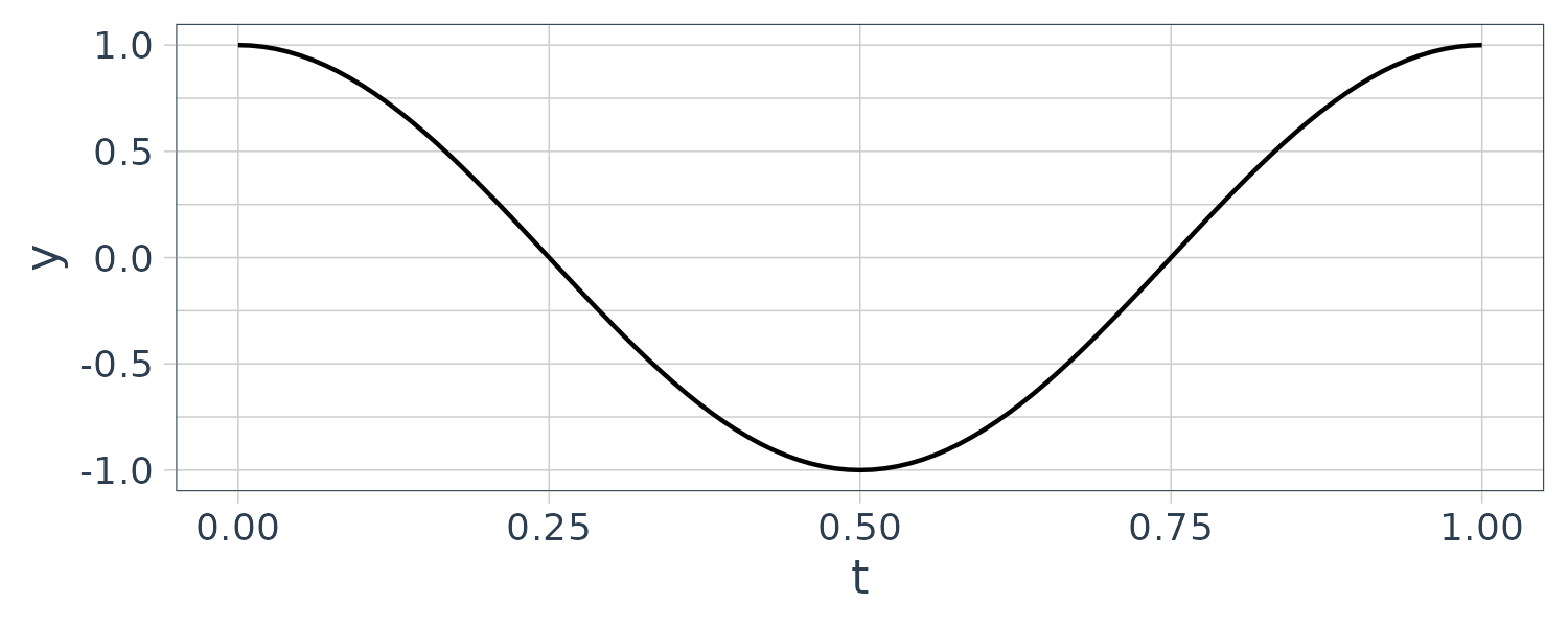
Next we will use R’s fft function to find the frequency component. Since cosine wave consists of only real parts, we shall only plot the real part:
fs <- length(t)
ffts <- Re(fft(y)) / fs
dat <- tibble(
  x = -10:10,
  fft = c(
    ffts[(51 + 40):100],
    ffts[1:(51 - 40)]
    )
)
dat |>
  ggplot() +
  geom_segment(mapping = aes(x = x, xend = x, y = 0, yend = fft)) +
  theme_tq()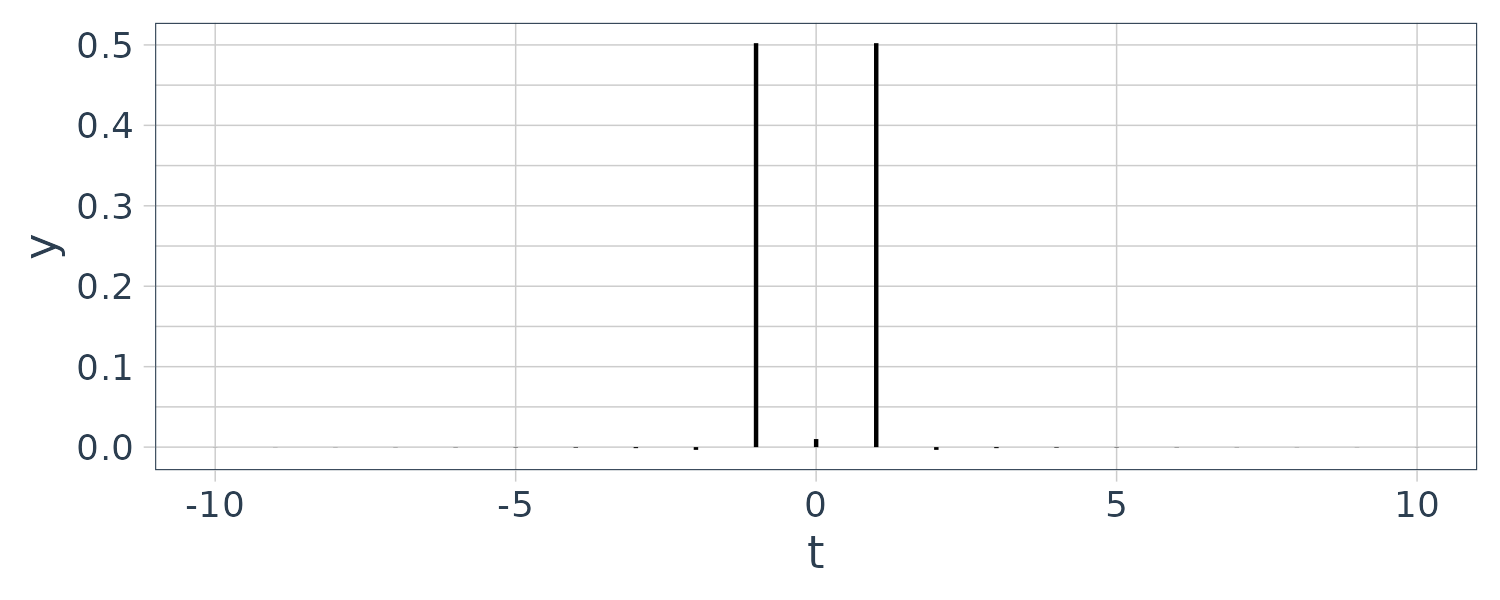
We will explain the fft function more during the Fourier Transform section. But note here that the fft function returns the vector in a way such that the negative part is tagged after the positive part so we need to do some vector manipulation to get it to graph correctly. Also I am only graphing -10:10 data points.
For the sine wave:
\[\begin{aligned} f(t) &= A\mathrm{sin}(\omega_{0}t)\\ &= \frac{A}{2i}e^{i\omega_{0}t} - \frac{A}{2i}e^{-i\omega_{0}t}\\ &= -\frac{Ai}{2}e^{i\omega_{0}t} + \frac{Ai}{2}e^{-i\omega_{0}t} \end{aligned}\]A <- 1
num_periods <- 1
f <- 1
t <- seq(0, f * num_periods, length = 100)
omega <- 2 * pi * f
y <- A * sin(omega * t)
tibble(
t = t,
y = y
) |>
ggplot(aes(x = t, y = y)) +
geom_line() +
theme_tq()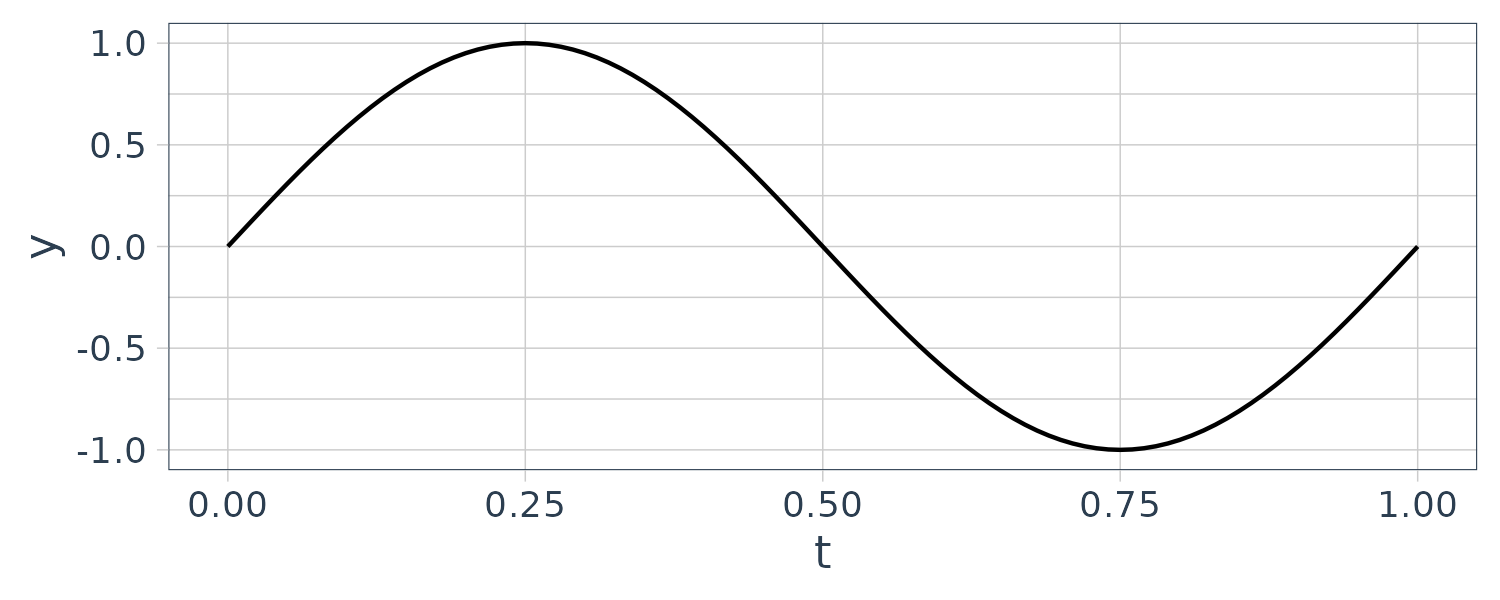
For the sine case, the two frequency components are \(\frac{A}{2i}\) and \(-\frac{A}{2i}\). We will graph the imaginary axis in this case:
fs <- length(t)
ffts <- Im(fft(y)) / fs
dat <- tibble(
  x = -10:10,
  fft = c(
    ffts[(51 + 40):100],
    ffts[1:(51 - 40)]
    )
)
dat |>
  ggplot() +
  geom_segment(mapping = aes(x = x, xend = x, y = 0, yend = fft)) +
  theme_tq()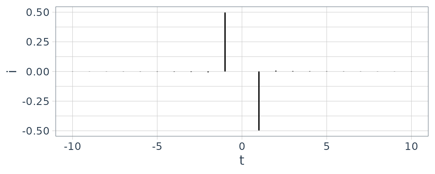
If we have both cosine and sine elements like below:
\[\begin{aligned} f(t) &= A\mathrm{cos}(\omega_{0}t) +A\mathrm{sin}(\omega_{0}t)\\ &= \frac{A}{2}e^{i\omega t} + \frac{A}{2}e^{-i\omega t} + \frac{A}{2i}e^{i\omega t} - \frac{A}{2i}e^{i\omega t}\\ &= \frac{A}{2}e^{i\omega t} + \frac{A}{2}e^{-i\omega t} - \frac{Ai}{2}e^{i\omega t} + \frac{Ai}{2}e^{i\omega t} \end{aligned}\]A <- 1
num_periods <- 1
f <- 1
t <- seq(0, f * num_periods, length = 100)
omega <- 2 * pi * f
y <- A * cos(omega * t) + A * sin(omega * t)
tibble(
t = t,
y = y
) |>
ggplot(aes(x = t, y = y)) +
geom_line() +
theme_tq()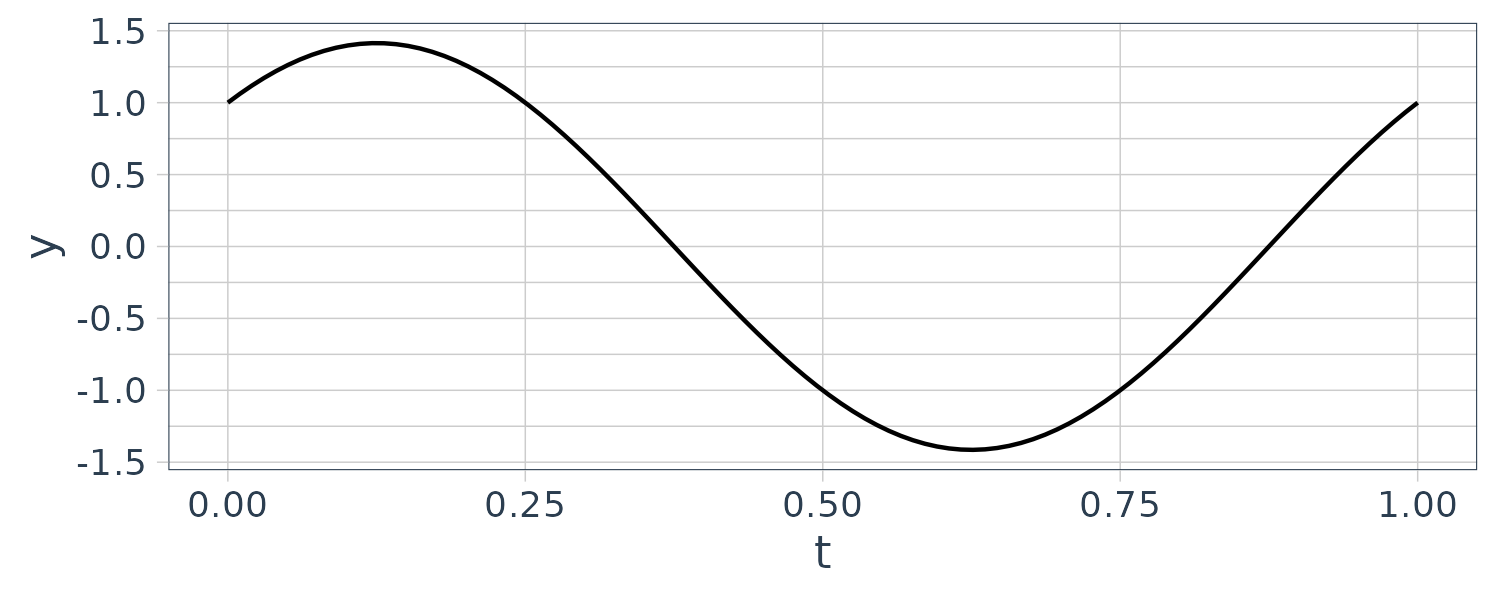
Will result in both real and imaginary amplitudes:
fs <- length(t)
ffts <- Re(fft(y)) / fs
dat <- tibble(
x = -10:10,
fft = c(
ffts[(52 + 40):101],
ffts[1:(51 - 40)]
)
)
dat |>
ggplot() +
geom_segment(mapping = aes(x = x, xend = x, y = 0, yend = fft)) +
xlab("t") +
ylab("y") +
theme_tq()
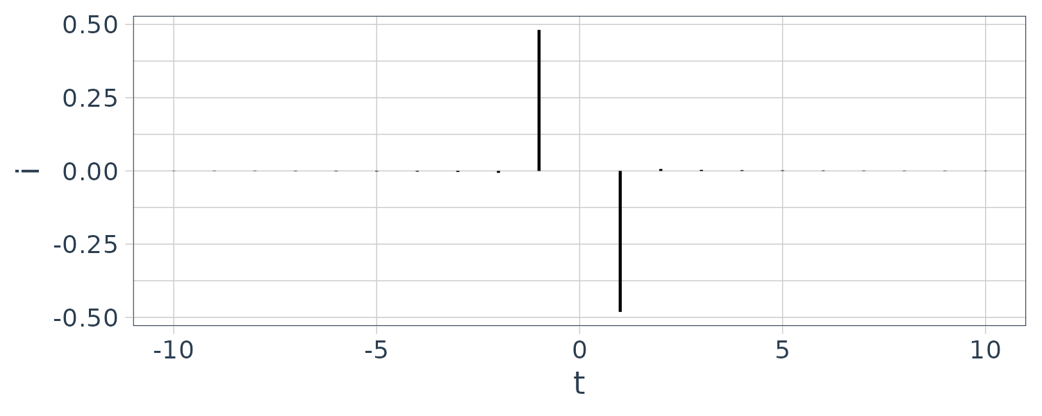
fs <- length(t)
ffts <- Im(fft(y)) / fs
dat <- tibble(
x = -10:10,
fft = c(
ffts[(51 + 40):100],
ffts[1:(51 - 40)]
)
)
dat |>
ggplot() +
geom_segment(mapping = aes(x = x, xend = x, y = 0, yend = fft)) +
xlab("t") +
ylab("y") +
theme_tq()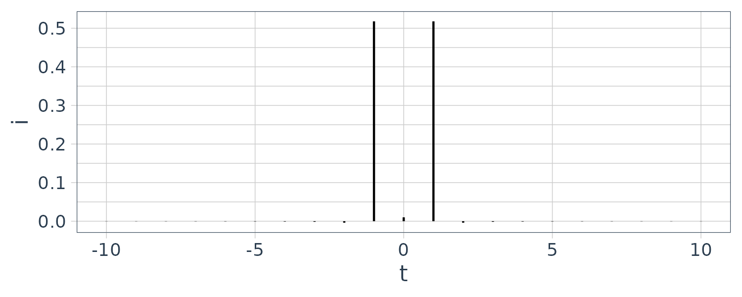
If we take the modulus of both the real and imaginary components:
\[\begin{aligned} \sqrt{\Big(\frac{A}{2}\Big)^{2} + \Big(\frac{A}{2}\Big)^{2}} &= \sqrt{\frac{A^{2}}{4} + \frac{A^{2}}{4}}\\ &= \sqrt{\frac{2A^{2}}{4}}\\ &= \sqrt{\frac{A^{2}}{2}}\\ &= \frac{A}{\sqrt{2}}\\ &= 0.7071 \end{aligned}\]And the phase:
\[\begin{aligned} \phi &= \mathrm{tan}^{-1}\Big(\frac{1}{1}\Big)\\ &= \frac{\pi}{4} \end{aligned}\]fs <- length(t)
ffts <- Mod(fft(y)) / fs
dat <- tibble(
x = -10:10,
fft = c(
ffts[(51 + 40):100],
ffts[1:(51 - 40)]
)
)
dat |>
ggplot() +
geom_segment(mapping = aes(x = x, xend = x, y = 0, yend = fft)) +
xlab("t") +
ylab("y") +
theme_tq()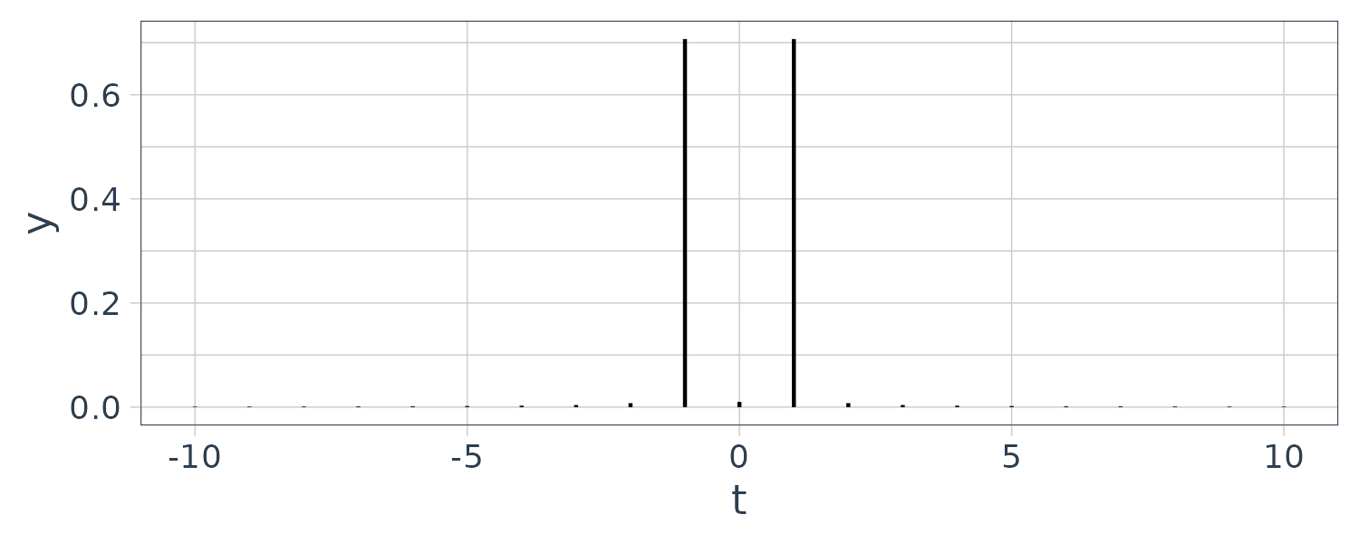
Note that the spectrum is only symmetric if the signal is real. If the signal is complex, the spectrum will be asymmetric. For example:
\[\begin{aligned} f(t) &= e^{i\omega t} \end{aligned}\]fs <- length(t)
ffts <- Mod(fft(y)) / fs
dat <- tibble(
x = -10:10,
fft = c(
ffts[(51 + 40):100],
ffts[1:(51 - 40)]
)
)
dat |>
ggplot() +
geom_segment(mapping = aes(x = x, xend = x, y = 0, yend = fft)) +
xlab("t") +
ylab("y") +
theme_tq()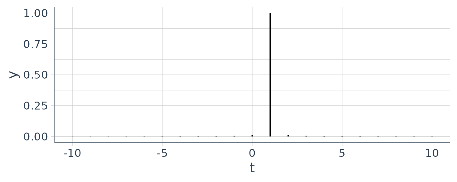
Shannon’s Theorem
Shannon’s theorem states that:
For any analog signal containing among its frequency content a maximum frequency of \(f_{max}\), then the analog signal can be represented faithfully by N equally spaced samples, provided the sampling rate is at least two times \(f_{max}\) samples per second.
Nyquist Frequency
Because of the concept known as aliasing, there is no way to detect any frequency higher than 2 times the samping frequency. Denoting the maximum frequency detectable as \(f_{max}\), the Nyquist rate is defined as:
\[\begin{aligned} F_{s} &= 2 f_{max} \end{aligned}\]What is usually done is to first identify \(f_{max}\) and then determining the appropriate sampling frequency \(F_{s}\):
\[\begin{aligned} F_{s} &\geq 2 f_{max} \end{aligned}\]Note that this is no direct relationship between \(F_{s}\) and the fundamental \(f_{0}\).
References
The Intuitive Guide to Fourier Analysis and Spectral Estimation: with Matlab
