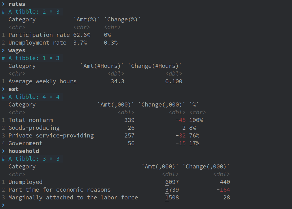
The Employment Situation report, aka Jobs report, aka Payroll report comes out the first Friday of the month at 8:30am EST. Revisions are monthly. In this post, we explain the key components of the report to look out for.

Also known as the Current Population Survey. The household survey attempts to measure labor force status and unemployment by demographic characteristics. 60,000 households are sampled across the US to be interviewed about work and job search. The survey week is usually conducted during the week containing the 19th of the month. The survey target the reference week containing the 12th of the month. The government will contact and interview the household with questions like:

Are you working?
Was the job full or part time?
If you are not working, how many weeks have you been unemployed?
How long have you been looking for work?
Did you make attempt to find work in the last four weeks?

The unemployment rate is listed in the report and calculated by dividing the number of unemployed workers by the labor force. The current unemployment rate is 3.4% with the labor participation rate at 62.6%.

Below are the list of tables found in the report:

Table A-1. Employment status of the civilian population by sex and age
Table A-2. Employment status of the civilian population by race, sex, and age
Table A-3. Employment status of the Hispanic or Latino population by sex and age
Table A-4. Employment status of the civilian population 25 years and over by educational attainment
Table A-5. Employment status of the civilian population 18 years and over by veteran status, period of service, and sex, not seasonally adjusted
Table A-6. Employment status of the civilian population by sex, age, and disability status, not seasonally adjusted
Table A-7. Employment status of the civilian population by nativity and sex, not seasonally adjusted
Table A-8. Employed persons by class of worker and part-time status
Table A-9. Selected employment indicators
Table A-10. Selected unemployment indicators, seasonally adjusted
Table A-11. Unemployed persons by reason for unemployment
Table A-12. Unemployed persons by duration of unemployment
Table A-13. Employed and unemployed persons by occupation, not seasonally adjusted
Table A-14. Unemployed persons by industry and class of worker, not seasonally adjusted
Table A-15. Alternative measures of labor underutilization
Table A-16. Persons not in the labor force and multiple jobholders by sex, not seasonally adjusted

Civilian Labor Force

The labor force is not as clear cut as it sounds. The civilian population consists only on 16 and above, and not on active military duty, and in some kind of institutional facility like mental hospitals and prisons. Also only those who are employed or those unemployed but are actively looking for a job are counted.

Therefore, to be categorized as unemployed, a person would have to be counted as part of the civilian workforce and jobless during the survey week.

Labor Force Participation Rate

The above Labor Force is then divided by the working civilian population to determine the proportion of the population actually employed. In other words, it shows how much of the population are discouraged workers or retirees.

In a typical business cycle, the participation rate will go up when the economy is robust, and similar a falling participation rate signal a faltering economy.

On average, about 150,000 new people reach the working age every month due to population growth, immigration, or students who graduate. Economists estimate GDP has to grow 3-4% just to produce enough employment for these new labors.

Employment Population Ratio

The above Labor Force divided by the whole country population is the employment-population ratio. It tells a similar story as the participation rate, but also indicate whether the economy is generating enough jobs for a growing population.

Establishment Survey (NonFarm Payrolls)

Also known as the Current Employment Statistics Survey. The establishment survey attempts to measure nonfarm employment, hours, and earnings by industry. the survey samples 440,000 nonfarm businesess and uses the same reference week (12th) as the Household Survey. Rather than contacting the household, the establishment survey gathers information directly from the business establishments which should be more accurate as household are more proned to lie in the interviews.

However, on average only 50% of the business response make it in time for the first release as they are prone to report late. Subsequent revisions for the next two months will bum up the the response rate to 80% and above.

The nonfarm payrolls fall into 3 categories:

Goods Producing (13%)
- Manufacturing Jobs (65%)
- Construction Jobs (30%)
- Mining and Logging Jobs (4%)
Private Service Providing (70%)
- Service Jobs (83%)
Government (17%)
- Local (65%)
- State (23%)
- Federal (12%)

Economists pay attention to the total non-farm and non-govermentpayrolls, which include just the goods and service sector.

Below are the list of tables found in the report:

Table B-1. Employees on nonfarm payrolls by industry sector and selected industry detail
Table B-2. Average weekly hours and overtime of all employees on private nonfarm payrolls by industry sector, seasonally adjusted
Table B-3. Average hourly and weekly earnings of all employees on private nonfarm payrolls by industry sector, seasonally adjusted
Table B-4. Indexes of aggregate weekly hours and payrolls for all employees on private nonfarm payrolls by industry sector, seasonally adjusted
Table B-5. Employment of women on nonfarm payrolls by industry sector, seasonally adjusted
Table B-6. Employment of production and nonsupervisory employees on private nonfarm payrolls by industry sector, seasonally adjusted(1)
Table B-7. Average weekly hours and overtime of production and nonsupervisory employees on private nonfarm payrolls by industry sector, seasonally adjusted(1)
Table B-8. Average hourly and weekly earnings of production and nonsupervisory employees on private nonfarm payrolls by industry sector, seasonally adjusted(1)
Table B-9. Indexes of aggregate weekly hours and payrolls for production and nonsupervisory employees on private nonfarm payrolls by industry sector, seasonally adjusted(1)

The data obtained from Establishment survey is also used in the construction of the “Personal Income and Outlays Report” and the “Industrial Production and Capacity Utilization Report”, which is used in the indexes of leanding and conincidental economic indicators.

Average Hourly Earnings

Average Hourly Earnings can be considered a proxy for inflation. It also correlates closely with GDP. It is often a leading indicator for more hiring or layoff.

When the average weekly manufacturing hours falls below 40 hours, it usually indicate the economy is faltering.

Phillips Curve

The relationship between inflation and unemployment is known as the Phillips curve. During the period studied, it was found out that low periods of unemployment coincide with high wage increases, and high periods of unemployment coincide with high unemployment. Therefore there seem to be a tradeoff between inflation and unemployment. The Phillips curve has broken down in recent years.

NAIRU

The Non-Accelerating-Inflation rate of unemployment (NAIRU), is the lowest level of unemployment without an increase in inflation. Also known as the natural unemployment rate (about 6%).

Unemployment Rate as a Leading Indicator

Unemployment tends to increase sharply just before a recession, and take several years for the unemployment rate to go down once the recession ends. Note that unemployment rate is not one of the indicator in The Conference Board LEI.

Differences Between the Surveys

The establishment survey has a smaller margin of error (MoM) due to its larger sample size. A MoM change of about 130,000 is considered statistically signifcant while for the household survey is about 600,000.

The Establishment job numbers tend to be higher than the Household, but they generally trend in the same direction. But sometimes they do give conflicting answers. The reason is because they measure slightly different things.

Household surveys only interview individuals who are 16 and above, include both farm and nonfarm workers. Also if the same individual hold multiple part time jobs, only employed person is counted. Establishment survey doesn’t make the distinction and counts all age group, and multiple jobs as multiple employments and only include nonfarm employments.

Household survey also includes sel-employed workers, unpaid family workers, agricultural workers, and private household workers that are excluded by the establishment survey.

Scrap Data

Let us now scrap some of the important information from the Employment Situation report using R:

url <- "https://www.bls.gov/news.release/empsit.a.htm"
page <- read_html(
  paste0(url)
)

household <- page |>
  html_nodes("#cps_empsit_sum") |>
  html_table() |>
  nth(1)

rates <- household

names(household)[5] <- "Amt(,000)"
names(household)[6] <- "Change(,000)"

names(rates)[5] <- "Amt(%)"
names(rates)[6] <- "Change(%)"

cols <- c(
  "Unemployed",
  "Part time for economic reasons",
  "Marginally attached to the labor force"
)
household <- household |>
  select(c(1, 5, 6)) |>
  mutate(
    `Amt(,000)` = as.numeric(gsub(",", "", `Amt(,000)`)),
    `Change(,000)` = as.numeric(gsub(",", "", `Change(,000)`))
  ) |>
  filter(Category %in% cols)

cols <- c(
  "Unemployment rate",
  "Participation rate"
)
rates <- rates |>
  select(c(1, 5, 6)) |>
  mutate(
    `Amt(%)` = paste0(as.numeric(gsub(",", "", `Amt(%)`)), "%"),
    `Change(%)` = paste0(as.numeric(gsub(",", "", `Change(%)`)), "%")
  ) |>
  filter(Category %in% cols)

url <- "https://www.bls.gov/news.release/empsit.b.htm"
page <- read_html(
  paste0(url)
)

est <- page |>
  html_nodes("#ces_table10") |>
  html_table() |>
  nth(1)

wages <- est

names(est)[4] <- "Prev(,000)"
names(est)[5] <- "Amt(,000)"

names(wages)[4] <- "Prev(#Hours)"
names(wages)[5] <- "Amt(#Hours)"

cols <- c(
  "Total nonfarm",
  "Goods-producing",
  "Private service-providing",
  "Government"
)

est <- est |>
  select(c(1, 4, 5)) |>
  mutate(
    `Prev(,000)` = as.numeric(gsub(",", "", gsub("\\$", "", `Prev(,000)`))),
    `Amt(,000)` = as.numeric(gsub(",", "", gsub("\\$", "", `Amt(,000)`)))
  ) |>
  mutate(
    `Change(,000)` = `Prev(,000)` - `Amt(,000)`
  ) |>
  select(-`Prev(,000)`) |>
  filter(Category %in% cols)

est <- est[!duplicated(est$Category), ]
total <- est |>
  filter(Category == "Total nonfarm") |>
  pull(`Amt(,000)`)

est <- est |>
  mutate(
    `%` = paste0(round((`Amt(,000)` / total) * 100), "%")
  )

cols <- c(
  "Average weekly hours"
)
wages <- wages |>
  select(c(1, 4, 5)) |>
  mutate(
    `Prev(#Hours)` = as.numeric(gsub(",", "", gsub("\\$", "", `Prev(#Hours)`))),       
    `Amt(#Hours)` = as.numeric(gsub(",", "", gsub("\\$", "", `Amt(#Hours)`)))
  ) |>
  mutate(
    `Change(#Hours)` = `Prev(#Hours)` - `Amt(#Hours)`
  ) |>
  select(-`Prev(#Hours)`) |>
  filter(Category %in% cols)