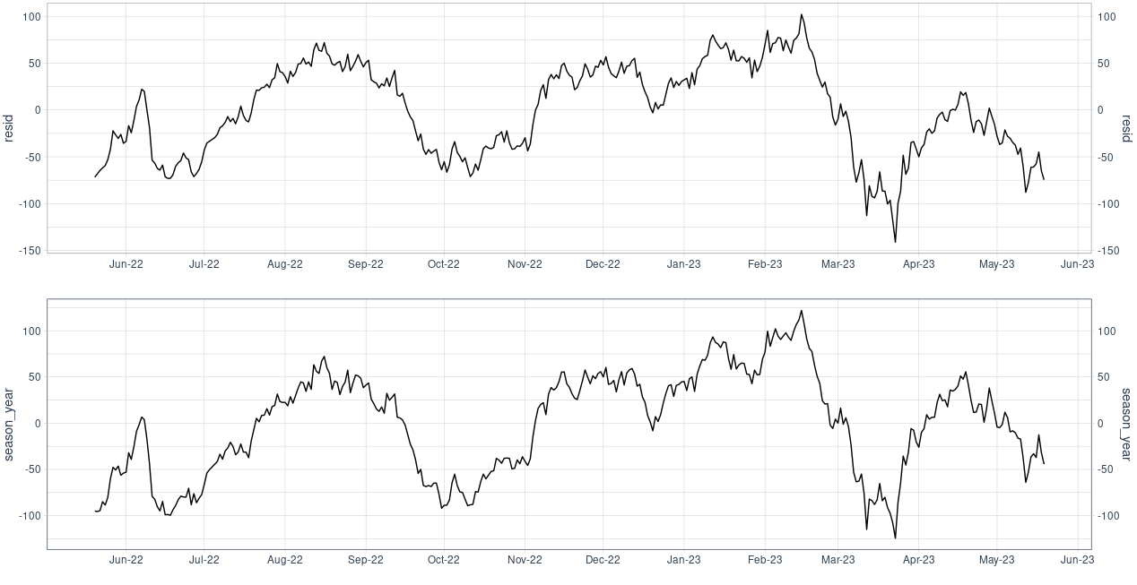
In this post, we are attempting to replicate STL seasonal component calculation. We will use S&P 500 close prices for demonstration.

Get Data

The first step would be to get the closing prices. As we are looking specifically at annual season, we would require a number of years to average the values for a particular day of the month. We arbitrary chose 7 years:

end <- Sys.Date()
start <- end - years(7)
prices <- getData("^GSPC", start, end, "daily") |>     
  as_tsibble(index = date) |>
  fill_gaps()

Because of weekends and public holidays and we are using daily data, we need to fill these gaps as NA values. But in the following code, we would use linear interpolation to fill them up with values:

prices$close <- prices |>
  model(naive = ARIMA(close ~ -1 + pdq(0, 1, 0) + PDQ(0, 0, 0))) |>     
  interpolate(prices) |>
  pull(close)

STL

STL stands for “Seasonal and Trend decomposition using Loess”. It decompose a time series data into a trend, seasonal, and remainder components. We will invoke STL to extract the seasonal component and in later sections replicate the result.

dcmp <- prices |>
  model(stl = STL(    
    close
  )) %>%
  components()

dcmp |>
  autoplot() +
  theme_tq()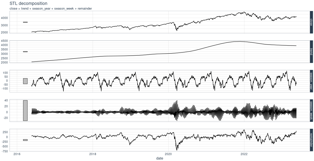

Seasonal Component

We will iterate in a loop for about 365 days, and average the values for the same day or the month across the 7 years in our data. We keep track of a year when the day and month is the same for the next year. This will inform us that we have finished a year worth of data. We will store the data in a tibble.

flag <- TRUE
init_day <- day(prices$date[1])
init_month <- month(prices$date[1])
init_year <- year(prices$date[1])
idx <- 1
avgs <- c()
res <- NULL
while(flag) {

  curr_day <- day(prices$date[idx])
  curr_month <- month(prices$date[idx])

  if (idx > 1) {
    if (curr_day == init_day & curr_month == init_month) {
      break
    }
  }

  avg <- prices |>
    filter(day(date) == curr_day & month(date) == curr_month) |>      
    pull(close) |>
    mean()

  avgs <- c(avgs, avg)

  row <- tibble(
    day = curr_day,
    month = curr_month,
    date = prices$date[idx] + years(7 - 1),
    avg = avg
  )

  if (is.null(res)) {
    res <- row
  } else {
    res <- rbind(res, row)
  }

  idx <- idx + 1
}

Once this is done, we need to detrend the averages and extract the residues. The easiest way is to fit a linear regression, followed by calling the resid() function:

fit <- lm(avg ~ as.numeric(date), data = res)     
res$resid <- residuals(fit)

Finally we plot the data and contrast it with what we get from STL:

fit <- lm(avg ~ as.numeric(date), data = res)     
res$resid <- residuals(fit)

We can see some differences, but the general up/down direction is the same. The tiny differences could be due to STL using a weighted average (giving more weights to years close to the current year).

See Also

References

Forecasting:Principles and Practice (Hyndman)