Yield Curve
Read Post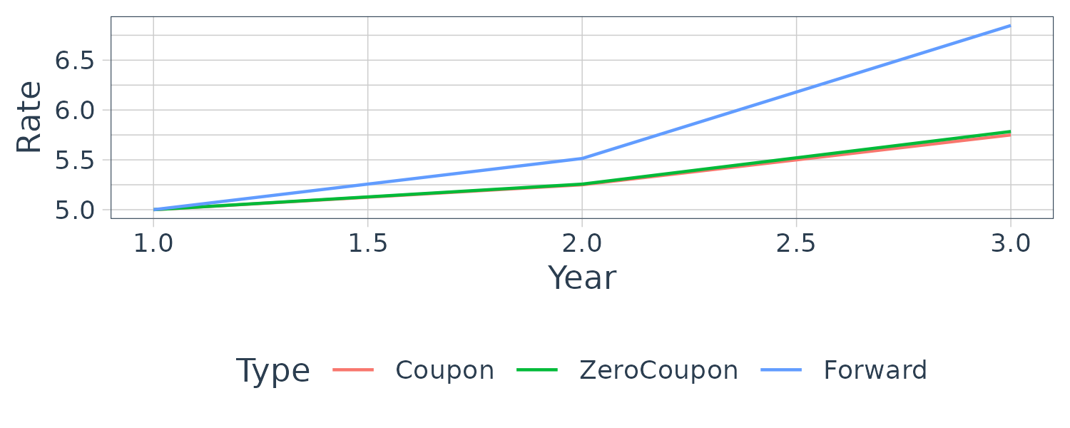
In this post we will talk about yield curve.
Contents:
Liquidity Preference Theory
Longer term bonds are less liquid and viewed to be riskier which command a liquidity premium from investors. Essentially the liquidity premium is always positive and given a constant inflation expectation (i.e. flat yield curve) would make the yield curve to be positively sloped.
Zero-Coupon Yield Curve
The dirty price of a bond when priced using a zero-coupon yield curve:
\[\begin{aligned} \text{Price}_{\text{Dirty}} &= \sum_{n = 1}^{N}\frac{C}{(1 + r_{n})^{n}} + \frac{P}{(1 + r_{N})N}\\ &= \sum_{n = 1}^{N}\frac{C}{(1 + r_{n})^{n}} \times df_{n} + P \times df_{N} \end{aligned}\]Where the discount factor (df) is defined as:
\[\begin{aligned} df_{n} &= \frac{1}{(1 + r_{n})^{n}} \end{aligned}\]Suppose a $100 nominal of a 5% 2Y bond (annual coupon) priced at par. It has a $5 cashflow at year 1 and a $105 cashflow at year 2. So effectively, it is equivalent to a 1Y $5 zero-coupon bond, and a 2Y $105 zero coupon bond.
Now, supposed a 1Y bond that pays a coupon of 5% is currently priced at par. In one year’s time, we will receive $105. So the interest is simply 5%.
Now, assume a 2Y bond that pays a coupon of 6% and is currently priced at $99. We can use the $99 to instead buy a 1Y bond at 5% giving a cashflow of:
\[\begin{aligned} 99 \times 1.05 &= 103.95 \end{aligned}\]Hence, we will get this 103.95 in 1 year’s time. The same 2Y bond will still continue to pay 6% for the next year. Hence, the 2y bond should cost now cost:
\[\begin{aligned} 103.95 - 6 &= 97.95 \end{aligned}\]This is because of the following relationship:
\[\begin{aligned} 99 &= \frac{6}{1.05} + \frac{106}{1.05\times(1 + {}_{1}f_{1})}\\[5pt] &= \frac{1}{1.05} \Big(6 + \frac{106}{1 + {}_{1}f_{1}}\Big) \end{aligned}\] \[\begin{aligned} 99 \times 1.05 &= 6 + \frac{106}{1 + {}_{1}f_{1}}\\[5pt] 103.95 - 6 &= \frac{106}{1 + {}_{1}f_{1}}\\[5pt] 97.95 &= \frac{106}{1 + {}_{1}f_{1}}\\[5pt] {}_{1}f_{1} &= \frac{106}{97.95} - 1\\[5pt] &= 8.22\% \end{aligned}\]The expected/equilibrium/implied forward rate is 8.22%. If an investor think the forward rate is higher, the investor would not buy the 2Y bond but instead buy the 1Y bond and wait for a year to invest in a higher yield. Similarly, if investor thinks the forward rate is lower, the investor would buy a 1Y bond, and wait for a year and buy another 1Y bond at a lower rate. So in equilibrum, the implied forward rate is the expected forward rate.
Discount Factors
We can think of a bond as an annuity that pays out the coupons and a zero-coupon bond that pays out the principal at expiration.
If the bond is trading at par:
\[\begin{aligned} 100 &= C \times \sum_{n = 1}^{N}df_{n} + 100 \times df_{N}\\ &= C \times A_{N} + 100 \times df_{N} \end{aligned}\]Where \(df_{N}\) is the fair price of a \(N\) year zero-coupon bond with a par value of $1.
\(A\) is the fair price of a $1 \(N\) year annuity:
\[\begin{aligned} A_{N} &= \sum_{n = 1}^{N}df_{n}\\ &= A_{N-1} + df_{N}\\ A_{0} &= 0 \end{aligned}\]Subsituting \(A_{N}\) into the bond equation:
\[\begin{aligned} 1 &= C \times (A_{N-1} + df_{N}) + 1 \times df_{N}\\ &= C \times A_{N-1} + C \times df_{N} + 1 \times df_{N}\\ &= C \times A_{N-1} + df_{N}(C + 1)\\ df_{N} &= \frac{1 - C \times A_{N - 1}}{C + 1} \end{aligned}\]For example if the 1Y, 2Y, and 3Y redemption yield at par is 5%, 5.25% and 5.275% respectively:
\[\begin{aligned} df_{1} &= \frac{1}{1 + 0.05}\\[5pt] &= 0.95238\\[5pt] df_{2} &= \frac{1 - 0.0525 \times 0.95238}{1 + 0.0525}\\[5pt] &= 0.90261\\[5pt] df_{3} &= \frac{1 - 0.0575 \times (0.95238 + 0.90261)}{1 + 0.0575}\\[5pt] &= 0.84476 \end{aligned}\]We can check that these discount factors are correct:
\[\begin{aligned} 100 &= 105 \times 0.95238\\ 100 &= (5.25 \times 0.95238) + (105.25 \times 0.90261)\\ 100 &= (5.75 \times 0.95238) + (5.75 \times 0.90261) + (105.75 \times 0.84476) \end{aligned}\]And calculating the spot yields:
\[\begin{aligned} df_{1} &= \frac{1}{1 + r_{1}}\\[5pt] &= 0.95238\\[5pt] df_{2} &= \frac{1}{(1 + r_{2})^{2}}\\[5pt] &= 0.90261\\[5pt] df_{3} &= \frac{1}{(1 + r_{3})^{3}}\\[5pt] &= 0.84476\\[5pt] \end{aligned}\] \[\begin{aligned} r_{1} &= 5.0\%\\ r_{2} &= 5.256\%\\ r_{3} &= 5.784\% \end{aligned}\]Forward Yield Curve
The relationship between spot and implied forward rates:
\[\begin{aligned} \text{Price}_{\text{Dirty}} &= \frac{C}{1 + {}_{0}f_{1}} + \frac{C}{(1 + {}_{0}f_{1})(1 + {}_{1}f_{2})} + \cdots + \frac{P}{(1 + {}_{0}f_{1})\cdots(1 + {}_{N-1}f_{N})}\\[5pt] &= \sum_{n = 1}^{N}\frac{C}{\prod_{n = 1}^{N}(1 + {}_{i-1}f_{i})} + \frac{P}{\prod_{n=1}^{N}(1 + {}_{i-1}f_{i})} \end{aligned}\] \[\begin{aligned} (1 + r_{n})^{n} &= (1 + {}_{0}f_{1})(1 + {}_{1}f_{2})\cdots(1 + {}_{n-1}f_{n}) \end{aligned}\] \[\begin{aligned} (1 + {}_{n-1}f_{n}) &= \frac{(1 + r_{n})^{n}}{(1 + r_{n-1})^{n-1}}\\[5pt] &= \frac{\frac{1}{df_{n}}}{\frac{1}{df_{n-1}}}\\[5pt] &= \frac{df_{n-1}}{df_{n}} \end{aligned}\]Using the earlier example where we calculated the zero-coupon spot rates as:
\[\begin{aligned} r_{1} &= 5.0\%\\ r_{2} &= 5.256\%\\ r_{3} &= 5.784\% \end{aligned}\] \[\begin{aligned} 1 + {}_{0}f_{1} &= 1 + r_{1}\\[5pt] &= 1.05\\[5pt] 1 + {}_{1}f_{2} &= \frac{(1 + 0.05256)^{2}}{1 + 0.05}\\[5pt] &= 1.055138\\[5pt] 1 + {}_{2}f_{3} &= \frac{(1 + 0.05778)^{3}}{(1 + 0.05265)^{2}}\\[5pt] &= 1.068479 \end{aligned}\] \[\begin{aligned} {}_{0}f_{1} &= 5.0\%\\ {}_{1}f_{2} &= 5.5138\%\\ {}_{2}f_{3} &= 6.8479\% \end{aligned}\]We can see from the graph below that for an upward sloping yield curve:
\[\begin{aligned} \text{Forward} > \text{Zero-Coupon} > \text{Coupon} \end{aligned}\]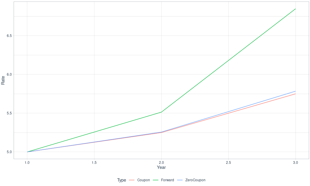
Note that of a upward sloping yield curve, we can only say that the forward rate will be above the spot yield curve. It is possible for the the forward rate curve to be decreasing and the spot yield curve to be still rising.
The general formula for forward rate from period \(a\) to \(b\) is:
\[\begin{aligned} {}_{a}f_{b} &= \Bigg(\frac{(1 + r_{b})^{b}}{(1 + r_{a})^{a}}\Bigg)^{\frac{1}{b-a}} - 1 \end{aligned}\]If the period a,b are less than one year (assuming DCF is 360):
\[\begin{aligned} {}_{a}f_{b} &= \Bigg(\frac{(1 + r_{b} \times \frac{b}{360}){1 + r_{a} \times \frac{a}{360}} - 1\Bigg) \times \frac{360}{b - a} \end{aligned}\]Bootstrapping
If \(d(t)\) is the t-year discount factor, a 5Y discount factor at a discount rate of 6%:
\[\begin{aligned} d(t) &= \frac{1}{(1 + r)^{t}}\\ d(5) &= \frac{1}{(1 + 0.06)^{5}}\\ &= 0.747258 \end{aligned}\]The set of discount factors for a time period is known as the “Discount Function”.
Suppose we have the following bonds:
| Coupon | Term (Years) | Price |
|---|---|---|
| 7% | 0.5 | 101.65 |
| 8% | 1 | 101.89 |
| 6% | 1.5 | 100.75 |
| 6.5% | 2 | 100.37 |
For a 7% coupon, we will get a coupon of \(\frac{7}{2} = 3.50\) and the following relationship:
\[\begin{aligned} d(0.5) \times (100 + 3.5) &= 101.65\\ d(0.5) &= 0.98213 \end{aligned}\]We move to the next bond:
\[\begin{aligned} 101.89 &= 4 \times d(0.5) + 104 \times d(1)\\ &= 4\times 0.98213 + 104 \times d(1)\\ d(1) &= 0.94194 \end{aligned}\]And so on:
\[\begin{aligned} 100.75 &= 3 \times d(0.5) + 3\times d(1) + 103 \times d(1.5)\\ d(1.5) &= 0.92211 \end{aligned}\] \[\begin{aligned} 100.37 &= 3.25 \times d(0.5) + 3.25\times d(1) + 3.25\times d(1.5) + 103.25 \times d(2)\\ d(2) &= 0.88252 \end{aligned}\]Once we have the discount function, we can easily calculate the spot rates and forward rates (see above sections).
More Examples
Break-Even Principle
A bank’s client wants to lock in the 1Y cost of borrowing in a year’s time. Consider the following spot yields:
\[\begin{aligned} r_{1} &= 10\%\\ r_{2} &= 12\% \end{aligned}\]To hedge and price this, the bank can borrow the funds for 2 years at 12% and invest for 1 year for 10%. The forward rate plus any spread will be the rate quote to the client.
\[\begin{aligned} (1 + r_{2})^{2} &= (1 + r_{1})(1 + {}_{1}f_{2})\\[5pt] {}_{1}f_{2} &= \frac{(1 + r_{2})^{2}}{1 + r_{1}} - 1\\[5pt] &= \frac{(1 + 0.12)^{2}}{1 + 0.10} - 1\\[5pt] &= 14.04\% \end{aligned}\]Forward Rate from Zero-Coupon Rate
A bank’s client to fix a 2Y yield he could issue in 3 year’s time. The following Treasury spot rates are:
\[\begin{aligned} r_{1} &= 6.25\%\\ r_{2} &= 6.75\%\\ r_{3} &= 7.00\%\\ r_{4} &= 7.125\%\\ r_{5} &= 7.25\% \end{aligned}\]The bank would hedge by borrowing for 5 years at 7.25% and investing the funds for 3 years:
\[\begin{aligned} \text{Total Cost of Funding} &= \text{Total Return on Investments}\\[5pt] (1 + r_{5})^{5} &= (1 + r_{3})^{3} \times (1 + {}_{3}f_{5})^{2}\\[5pt] (1 + {}_{3}f_{5})^{2} &= \frac{(1 + 0.0725)^{5}}{(1 + 0.0700)^{3}}\\[5pt] {}_{3}f_{5} &= \sqrt{\frac{(1 + 0.0725)^{5}}{(1 + 0.0700)^{3}}} - 1\\[5pt] &= 7.63\% \end{aligned}\]Funding Gap
Consider a bank positions:
- Borrowing of 100 mio for 30 days at 5.875%
- Loan of 100 mio for 60 days at 6.125%
To hedge this funding gap, the bank can deal at the following forward rate (through FRA/futures):
\[\begin{aligned} {}_{30D}f_{60D} &= \Bigg(\frac{(1 + r_{60D} \times 60/360)}{(1 + r_{30D} \times 30/360)} - 1\Bigg) \times \frac{360}{60 - 30}\\ &= 6.3443\% \end{aligned}\]Expectations Hypothesis
There are two versions of the expectation hypothesis.
Local Expectations Hypothesis
Local Expectation Hypothesis states that bonds of the same class have the same expected holding period return regardless of maturity. This suggests that a 6M bond and a 20Y bond will have the same period return on average. We will see later that in practice, long-dated term (riskier) bonds will on average have higher returns than short-dated bonds. This hypothesis however doesn’t explain the shape of the curve.
The Unbiased Expectations Hypothesis
The more popular Unbiased Expectations Hypothesis states that current implied forward rates are unbiased estimators of future spot interest rates. In other words, the longer term interest rate is a geometric average of expected future short-term rates:
\[\begin{aligned} (1 + r_{N})^{N} &= (1 + r_{1})(1 + {}_{1}f_{2})\cdots(1 + {}_{N-1}f_{N})\\ &= (1 + r_{N-1})^{N-1}(1 + {}_{N-1}f_{N}) \end{aligned}\]This hypothesis can be used to explain any realistic curve shapes. A rising yield curve is due to the expectation of future rise in short-term interest rates. Similarly, an inverted yield curve indicates an expectation of future false in short-term rates. However, studies (Fama 1976) have shown that the forward rates are biased upwards and tend to over-estimate future rates.
