In this post, we talk about Time Series Analysis.

Datasets

Let us look at the datasets we will be using in this post. All the datasets can be found in the astsa package.

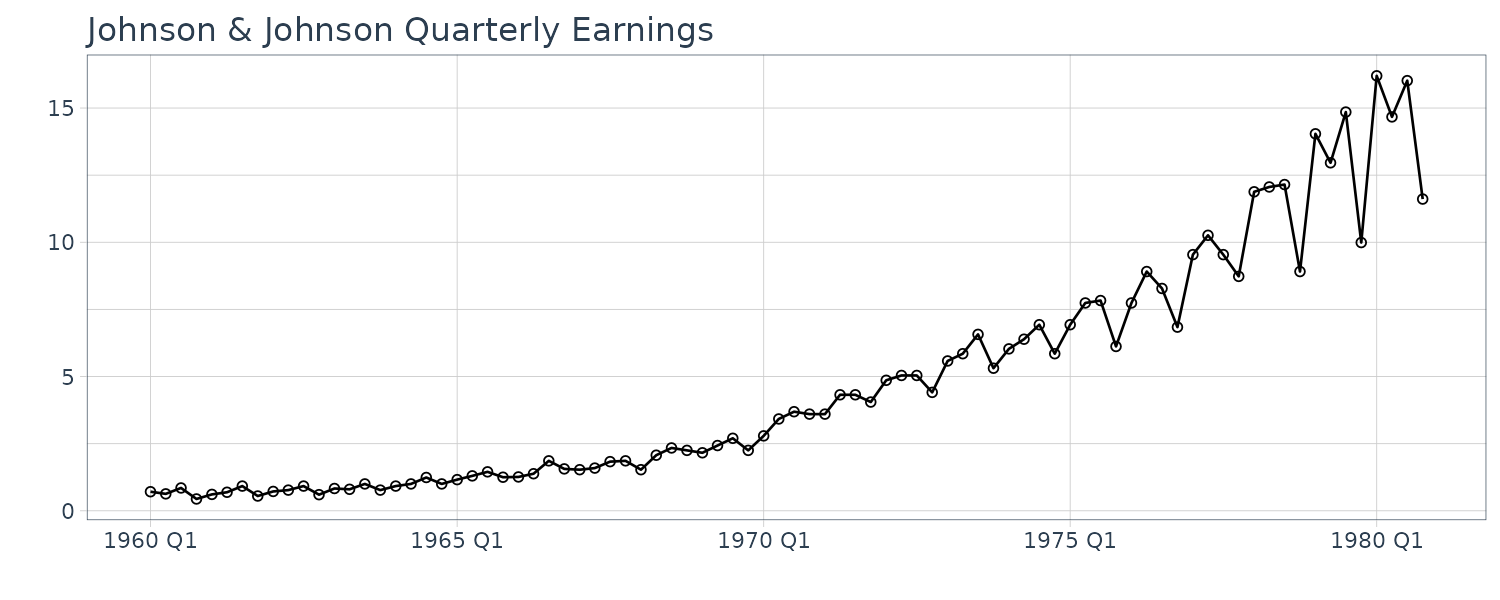
Johnson & Johnson Quarterly Earnings

Quarterly earnings per share of Johnson $ Johnson from 1960 to 1980 for a total of 84 quarters (21 years).

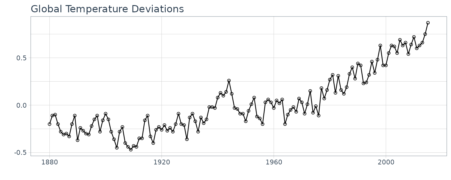
Global Warming

Global mean land-ocean temperature index from 1880 to 2015, with base period 1951-1980. The index is computed as deviation from the 1951-1980 average.

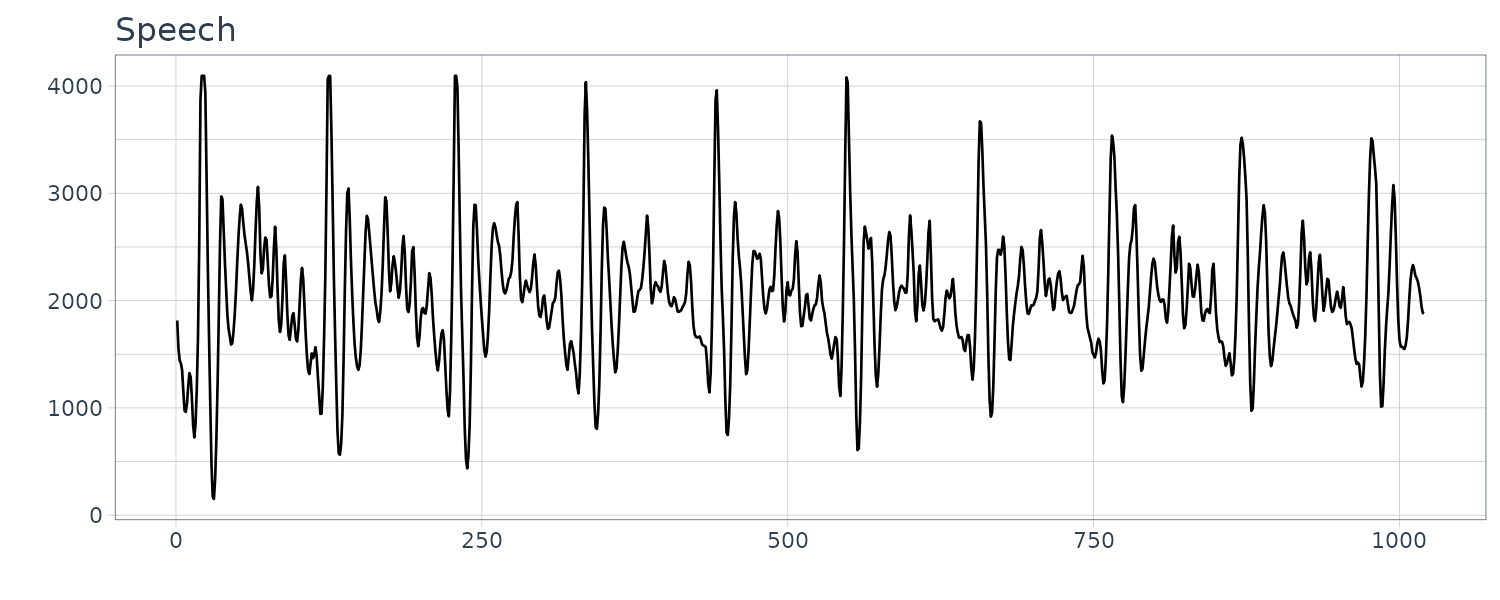
Speech Data

A 0.1 sec 1000 point sample of recorded speech for th eprhase “aahhhh”.

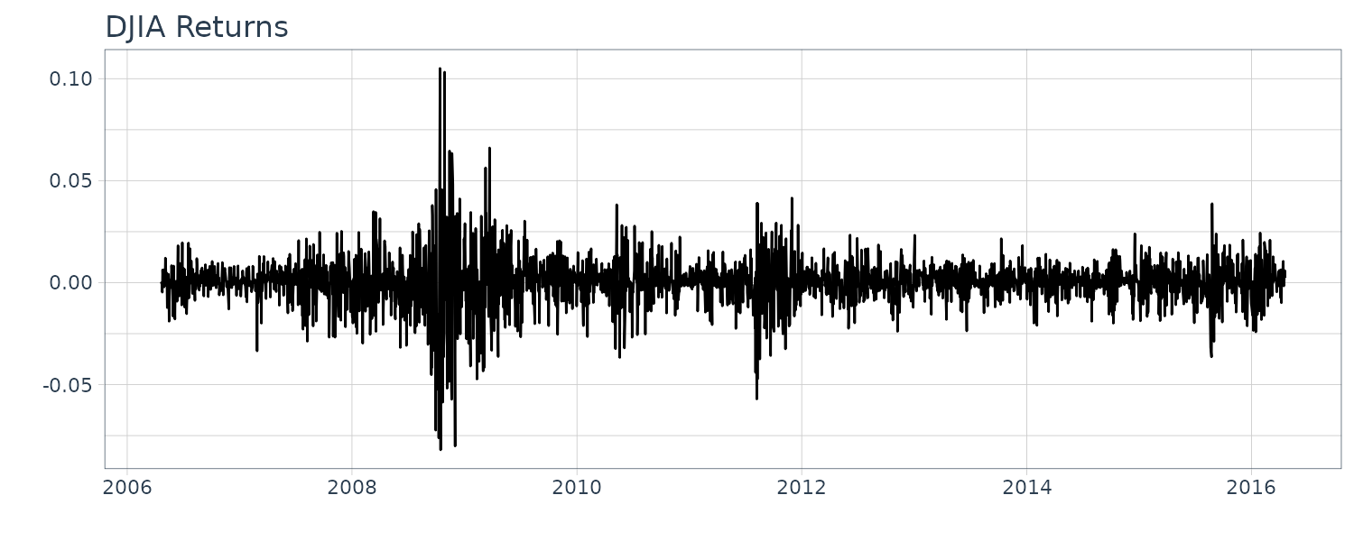
Dow Jones Industrial Average (DJIA)

Daily returns of the DJIA index from April 20, 2006 to April 20, 2016.

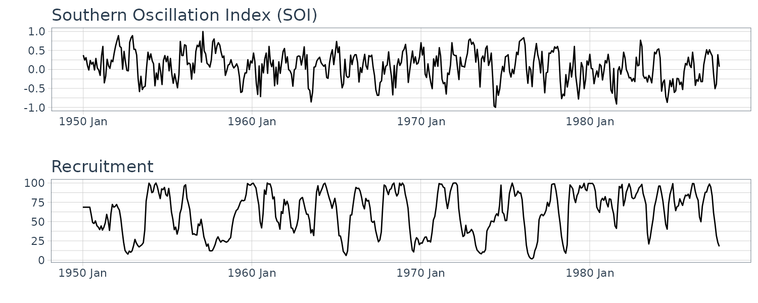
El Niño and Fish Population

Monthly values of the Southern Oscillation Index (SOI) and associated Recruitment (number of new fish) index ranging over the years 1950-1987. SOI measures changes in air pressure.

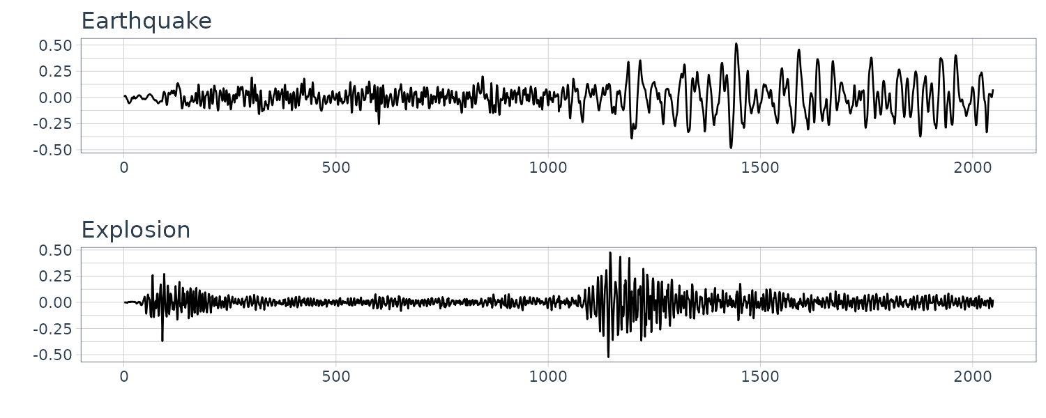
Earthquakes and Explosions

Seismic recording of an earthquake and explosion.

fMRI Imagining

Data is collected from various locations in the brain via Functional Magnetic Reasonance Imaging. A stimulus was applied for 32s and then stopped for 32 secs giving a total signal period of 64s. 1 observation is taken every 2s for 256s (n = 128).

Autocovariance

The autocovariance function is defined as:

\[\begin{aligned} \gamma_{x}(s, t) &= \mathrm{cov}(x_{s}, x_{t})\\ &= E[(x_{s} - \mu_{s})(x_{t} - \mu_{t})] \end{aligned}\]

Autocovariance function measures the linear dependence between two points in time. Smooth series have large autocovariance function even when \(s, t\) are far apart, whereas choppy series tend to have autocovariance function near 0.

If the random variables are linear combinations of \(X_{j}\) and \(Y_{k}\):

\[\begin{aligned} U &= \sum_{j=1}^{m}a_{j}X_{j}\\ V &= \sum_{k = 1}^{r}b_{k}Y_{k}\\ \mathrm{cov}(U, V) &= \sum_{j = 1}^{m}\sum_{k = 1}^{r}a_{j}b_{k}\mathrm{cov}(X_{j}, Y_{k}) \end{aligned}\]

If \(x_{s}, x_{t}\) are bivariate normal, \(\gamma_{x}(s, t) = 0\) implies independence as well.

And the variance:

\[\begin{aligned} \gamma_{x}(t, t) &= E[(x_{t} - \mu_{t})^{2}]\\ &= \mathrm{var}(x_{t}) \end{aligned}\]

The variance of a linear combination of \(x_{t}\) can be represented as sum of autocovariances:

\[\begin{aligned} \mathrm{var}(a_{1}x_{1} + \cdots + a_{n}x_{n}) &= \mathrm{cov}(a_{1}x_{1} + \cdots + a_{n}x_{n}, a_{1}x_{1} + \cdots + a_{n}x_{n})\\ &= \sum_{j= 1}^{n}\sum_{k = 1}^{n}a_{j}a_{k}\mathrm{cov}(x_{j}, x_{k})\\ &= \sum_{j= 1}^{n}\sum_{k = 1}^{n}a_{j}a_{k}\gamma(j - k) \end{aligned}\]

Note that:

\[\begin{aligned} \gamma(h) &= \gamma(-h) \end{aligned}\]

The autocorrelation function (ACF) is defined as:

\[\begin{aligned} \rho(s, t) &= \frac{\gamma(s, t)}{\sqrt{\gamma(s, s)\gamma(t, t)}} \end{aligned}\]

The cross-covariance function between two time series, \(x_{t}\) and \(y_{t}\):

\[\begin{aligned} \gamma_{xy}(s, t) &= \mathrm{cov}(x_{s}, y_{t})\\ &= E[(x_{s} - \mu_{xs})(y_{t} - \mu_{yt})] \end{aligned}\]

And the cross-correlation function (CCF):

\[\begin{aligned} \rho_{xy}(s, t) &= \frac{\gamma_{xy}(s, t)}{\sqrt{\gamma_{x}(s, s)\gamma_{y}(t, t)}} \end{aligned}\]

Estimating Correlation

In most situation, we only have a single realization (sample) to estimate the population means and covariance functions.

To estimate the mean, we use the sample mean:

\[\begin{aligned} \bar{x} &= \frac{1}{n}\sum_{t=1}^{n}x_{t} \end{aligned}\]

The variance of the mean:

\[\begin{aligned} \mathrm{var}(\bar{x}) &= \mathrm{var}\Big(\frac{1}{n}\sum_{t=1}^{n}x_{t}\Big)\\ &= \sum_{j=1}^{n}\sum_{k=1}^{n}\frac{1}{n}\frac{1}{n}\mathrm{cov}(x_{j}, x_{k})\\ &= \frac{1}{n^{2}}\mathrm{cov}\Big(\sum_{t=1}^{n}x_{t},\sum_{t=1}^{n}x_{t} \Big)\\ &= \frac{1}{n^{2}}\Big(n \gamma_{x}(0) + (n-1)\gamma_{x}(1) + \cdots + \gamma_{x}(n-1) + (n-1)\gamma_{x}(-1) + (n-2)\gamma_{x}(-2) + \cdots + \gamma_{x}(1 - n)\Big)\\ &= \frac{1}{n}\sum_{h=-n}^{n}\Big(1 - \frac{|h|}{n}\Big)\gamma_{x}(h) \end{aligned}\]

If the process is white noise, the variance would reduce to:

\[\begin{aligned} \mathrm{var}(\bar{x}) &= \frac{1}{n}\gamma_{x}(0)\\ &= \frac{\sigma_{x}^{2}}{n} \end{aligned}\]

Sample Autocovariance Function

The sample autocovariance function is defined as:

\[\begin{aligned} \hat{\gamma}(h) &= \frac{1}{n}\sum_{t=1}^{n-h}(x_{t+h} - \bar{x})(x_{t} - \bar{x}) \end{aligned}\]

Note that the estimator above divides by \(n\) instead of \(n-h\). This guarantee that the variance is never negative:

\[\begin{aligned} \hat{\mathrm{cov}}(a_{1}x_{1} + \cdots + a_{n}x_{n}) &= \sum_{j=1}^{n}\sum_{k = 1}\hat{\gamma}(j-k) \end{aligned}\]

But note that neighter dividing by \(n\) or \(n-h\) result in an unbiased estimator of \(\gamma(h)\).

Similarly, the sample ACF is defined as:

\[\begin{aligned} \hat{\rho}(h) &= \frac{\hat{\gamma}(h)}{\hat{\gamma}(0)} \end{aligned}\]

Using R to calculate ACF:

> ACF(soi, value) |>      
  slice(1:6) |>
  pull(acf) |>
  round(3)
[1]  0.604  0.374  0.214  0.050 -0.107 -0.187

Large-Sample Distribution of ACF

If \(x_{t}\) is white noise, then for large \(n\), the sample ACF is approximately normally distributed with 0 mean and sd:

\[\begin{aligned} \sigma_{\hat{\rho}_{x}(h)} &= \frac{1}{\sqrt{n}} \end{aligned}\]

The larger the sample-size \(n\), the smaller standard deviation.

An example of ACF of speech dataset:

speech |>
  ACF(value, lag_max = 250) |>      
  autoplot() +
  xlab("") +
  theme_tq() +
  ggtitle("Speech")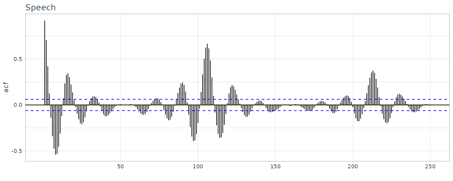

Sample Cross-Covariance Function

\[\begin{aligned} \hat{\gamma}_{xy}(h) &= \frac{1}{n}\sum_{t=1}^{n-h}(x_{t+h} - \bar{x})(y_{t} - \bar{y}) \end{aligned}\]

And the sample CCF:

\[\begin{aligned} \hat{\rho}_{xy}(h) &= \frac{\hat{\rho}_{xy}(h)}{\sqrt{\hat{\gamma}_{x}(0)\hat{\gamma}_{y}(0)}} \end{aligned}\]

Large-Sample Distribution of Cross-Correlation

If at least one of the processes is independent white noise:

\[\begin{aligned} \sigma_{\hat{\rho}_{xy}} &= \frac{1}{\sqrt{n}} \end{aligned}\]

Prewhitening and Cross Correlation Analysis

In order to test for cross linear dependence, at least one of the series must be white noise. To show as example, we generate two series:

\[\begin{aligned} x_{t} &= 2\mathrm{cos}(2\pi t \frac{1}{12}) + w_{t1}\\ y_{t} &= 2\mathrm{cos}(2\pi (t+5) \frac{1}{12}) + w_{t2}\\ \end{aligned}\]

If you look at the CCF:

set.seed(1492)
num <- 120
t <- 1:num
dat <- tsibble(
  t = t,
  X = 2 * cos(2 * pi * t / 12) + rnorm(num),
  Y = 2 * cos(2 * pi * (t + 5) / 12) + rnorm(num),      
  index = t
)

dat |>
  CCF(Y, X) |>
  autoplot() +
  ggtitle("CCF(X, Y)") +
  theme_tq()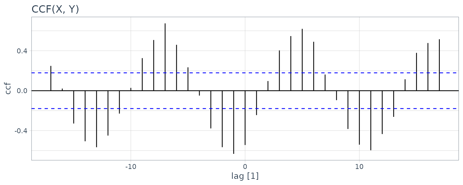

There appears to be cross-correalation between the sampe CCF although we know that the two series are independent.

To prewhiten \(y_{t}\) and plot the cross-correlation:

dat <- dat |>
  mutate(
    Yw = resid(lm(Y ~ cos(2 * pi * t / 12) + sin(2 * pi * t / 12), na.action = NULL))      
  )

dat |>
  CCF(Yw, X) |>
  autoplot() +
  ggtitle("CCF(X, Y)") +
  theme_tq()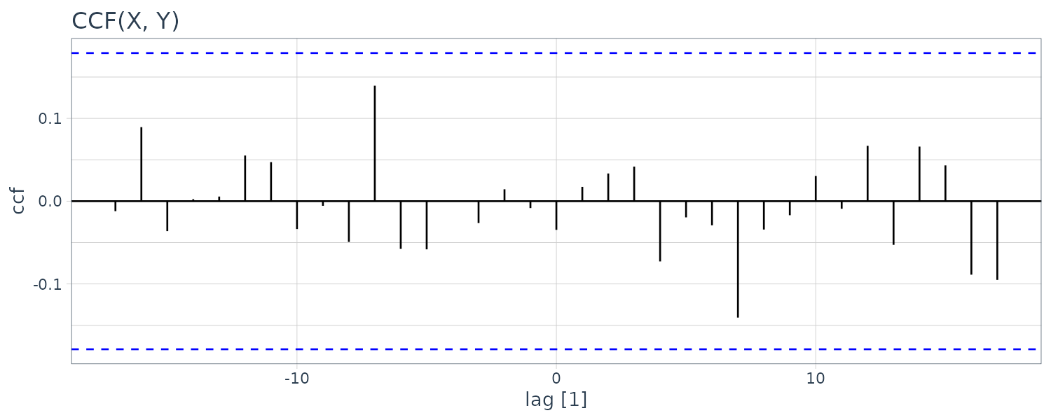

We can see that the cross-correlation is now insignificant.

Stationary Time Series

A strictly stationary time series has the same probability distribution when shifted by \(h\) for all \(k = 1, 2, \cdots\):

\[\begin{aligned} P(x_{t1} \leq c_{1}, \cdots, x_{tk} \leq c_{k}) &= P(x_{t1 + h} \leq c_{1}, \cdots, x_{tk + h} \leq c_{k}) &= \end{aligned}\]

Usually the strictly stationary condition is too imposing and a weaker version that only impose the first two moments of a seies is known as a “weakly statoionary” time series such that:

\[\begin{aligned} E[x_{t}] &= \mu_{t}\\ &= \mu\\ \gamma(t + h, t) &= \mathrm{cov}(x_{t + h}, x_{t})\\ &= \mathrm{cov}(x_{h}, x_{0})\\ &= \gamma(h, 0) \end{aligned}\]

In other words, the autocovariance function can be written as:

\[\begin{aligned} \gamma(h) &= \mathrm{cov}(x_{t+h}, x_{t})\\ &= E[(x_{t+h} - \mu)(x_{t} - \mu)] \end{aligned}\]

And the ACF:

\[\begin{aligned} \rho(h) &= \frac{\gamma(t+h, t)}{\sqrt{\gamma(t+h, t+h)\gamma(t, t)}}\\[5pt] &= \frac{\gamma(h)}{\gamma(0)} \end{aligned}\]

Jointly Staitonary

Two stationary time series\(x_{t}\) and \(y_{t}\) are said to be jointly stationary if the cross-covariance function:

\[\begin{aligned} \gamma_{xy}(h) &= \mathrm{cov}(x_{t+h}, y_{t})\\ &= E[(x_{t+h} - \mu_{x})(y_{t} - \mu_{y})] \end{aligned}\]

The CCF:

\[\begin{aligned} \rho_{xy}(h) &= \frac{\gamma_{xy}(h)}{\sqrt{\gamma_{x}(0)\gamma_{y}(0)}} \end{aligned}\]

In general,

\[\begin{aligned} \rho_{xy}(h) &\neq \rho_{xy}(-h)\\ \rho_{xy}(h) &= \rho_{yx}(-h) \end{aligned}\]

For example, if:

\[\begin{aligned} x_{t} &= w_{t} + w_{t-1}\\ y_{t} &= w_{t} - w_{t-1} \end{aligned}\] \[\begin{aligned} \gamma_{x}(0) &= 2\sigma_{w}^{2}\\ \gamma_{y}(0) &= 2\sigma_{w}^{2}\\ \gamma_{x}(1) &= \sigma_{w}^{2}\\ \gamma_{y}(1) &= -\sigma_{w}^{2} \end{aligned}\]

We can show that the autocovariance function depend only on the lag \(h\) and hence jointly stationary:

\[\begin{aligned} \gamma_{xy}(1) &= \mathrm{cov}(x_{t+1}, y_{t})\\ &= \mathrm{cov}(w_{t+1} + w_{t}, w_{t} - w_{t-1})\\ &= \sigma_{w}^{2} \end{aligned}\]

CCF:

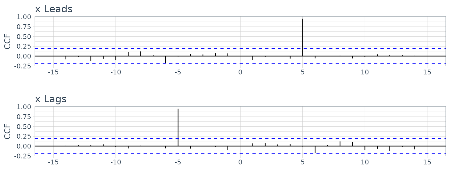
\[\begin{aligned} \rho_{xy}(h) &= \begin{cases} 0 & h = 0\\ \frac{1}{2} & h = 1\\ -\frac{1}{2} & h = -1\\ 0 & |h| \geq 2 \end{cases} \end{aligned}\]

Another example of cross-correlation where one series lead/lag another series. For the following model:

\[\begin{aligned} y_{t} &= Ax_{t-l} + w_{t} \end{aligned}\]

If \(l > 0\), \(x_{t}\) is said to lead \(y_{t}\) and if \(l < 0\), \(x_{t}\) is said to lag \(y_{t}\). Assuming \(w_{t}\) is uncorrelated with the \(x_{t}\) series, the cross-covariance function:

\[\begin{aligned} \gamma_{yx}(h) &= \mathrm{cov}(y_{t+h}, x_{t})\\ &= \mathrm{cov}(A x_{t+h - l} + w_{t+h}, x_{t})\\ &= \mathrm{cov}(A x_{t+h - l}, x_{t})\\ &= A\gamma_{x}(h - l) \end{aligned}\]

\(\gamma_{x}(h - l)\) will peak when \(h - l = 0\):

\[\begin{aligned} \gamma_{x}(h - l) &= \gamma_{x}(0) \end{aligned}\]

If \(x_{t}\) leads \(y_{t}\), the peak will be on the positive side and vice versa.

x <- rnorm(100)
dat <- tsibble(
  t = 1:100,
  x = x,
  y1 = stats::lag(x, -5) + rnorm(100),      
  y2 = stats::lag(x, 5) + rnorm(100),
  index = t
)

plot_grid(
  dat |>
    CCF(
      x,
      y1,
      lag_max = 15
    ) |>
    autoplot() +
    ylab("CCF Leads")
    xlab("") +
    theme_tq(),
  dat |>
    CCF(
      x,
      y2,
      lag_max = 15
    ) |>
    autoplot() +
    ylab("CCF Lags")
    xlab("") +
    theme_tq(),
  ncol = 1
)

Linear Process

A linear process, \(x_{t}\), is defined to be a linear combination of white noise variates \(w_{t}\):

\[\begin{aligned} x_{t} &= \mu + \sum_{j = -\infty}^{\infty}\psi_{j}w_{t-j}\\ \sum_{j=-\infty}^{\infty}|\psi_{j}| &< \infty \end{aligned}\]

The autocovariance can be shown to be:

\[\begin{aligned} \gamma_{x}(h) &= \sigma_{w}^{2}\sum_{j=-\infty}^{\infty}\psi_{j+h}\psi_{j} \end{aligned}\]

For a causal linear process, the processes do not depend on the future and we will have:

\[\begin{aligned} \psi_{j} &= 0\\ j &< 0 \end{aligned}\]

Gaussian Process

A process, \(\{x_{t}\}\), is said to be a Gaussian process if the n-dimensional \(\mathbf{x} = (x_{t1}, x_{t2}, \cdots, x_{tn})\) have a multivariate normal distribution.

Defining the mean and variance to be:

\[\begin{aligned} E[\mathbf{x}] &\equiv \mathbf{\mu}\\ &= \begin{bmatrix} \mu_{t1}\\ \mu_{t2}\\ \vdots\\ \mu_{tn} \end{bmatrix}\\[5pt] \mathrm{var}(\mathbf{x}) &\equiv \Gamma\\ &= \{\gamma(t_{i}, t_{j}); i, j = 1, \cdots, n\} \end{aligned}\]

The multivariate normal density function can then be written as:

\[\begin{aligned} f(\mathbf{x}) &= (2\pi)^{-\frac{n}{2}}|\Gamma|^{-\frac{1}{2}}e^{\frac{1}{2}(\mathbf{x} - \mathbf{\mu})^{T}\Gamma^{-1}(\mathbf{x}- \mathbf{\mu})} \end{aligned}\]

If the Gaussian time series, \(x_{t}\), is weakly stationary, then \(\mu_{t}\) is constant and:

\[\begin{aligned} \gamma(t_{i}, t_{j}) = \gamma(|t_{i} - t_{j}|) \end{aligned}\]

So that the vector \(\mathbf{\mu}\) and matrix \(\Gamma\) are independent of time and consist of constant values.

Note that it is not enough for the marginal distributions to be Gaussian in order for the joint distribution to be Gaussian.

Wold Decomposition

Wold Decomposition states that a stationary non-determinstic time series is a causal linear process:

\[\begin{aligned} x_{t} &= \mu + \sum_{j = 0}^{\infty}\psi_{j}w_{t-j}\\ \sum_{j=0}^{\infty}|\psi_{j}| &< \infty \end{aligned}\]

If the linear process is Gaussian, then:

\[\begin{aligned} w_{t} \sim \text{iid} N(0, \sigma_{w}^{2}) \end{aligned}\]

Time Series Statistical Models

White Noise

A collection of uncorrelated random variables with mean 0 and finite variance. Additionally, we require the random variables to be iid. If the RV is further Gaussian then:

\[\begin{aligned} w_{t} \sim N(0, \sigma_{\omega}^{2}) \end{aligned}\]

Autocovariance function:

\[\begin{aligned} \gamma_{w}(s, t) &= \mathrm{cov}(w_{s}, w_{t})\\ &= \begin{cases} \sigma_{w}^{2} & s = t\\ 0 & s \neq t \end{cases} \end{aligned}\]

Because white noise is weakly stationary, we can represent it in terms of lag \(h\):

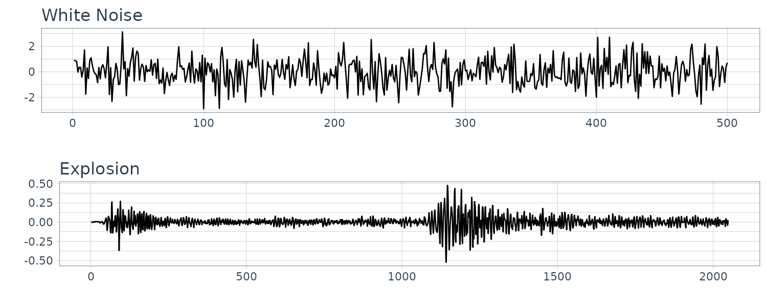
\[\begin{aligned} \gamma_{w}(h) &= \mathrm{cov}(w_{t + h}, w_{t})\\ &= \begin{cases} \sigma_{w}^{2} & h = 0\\ 0 & h \neq 0 \end{cases} \end{aligned}\]

The explosion series bears a slight resemblance to white noise:

dat <- tsibble(
  w = rnorm(500, 0, 1),
  t = 1:500,
  index = t
)
plot_grid(
  dat |>
    autoplot(w) +
    xlab("") +
    ggtitle("White Noise") +      
    theme_tq(),
  dat |>
    autoplot(v) +
    xlab("") +
    ggtitle("Explosion") +
    theme_tq(),
  ncol = 1
)

Moving Averages

To introduce serial correlation into the time series, we can replace the white noise series by a moving average that smooths out the series:

\[\begin{aligned} \nu_{t} = \frac{1}{3}(w_{t-1} + w_{t} + w_{t+1}) \end{aligned}\]

And the mean:

\[\begin{aligned} \mu_{\nu t} &= E[\nu_{t}]\\ &= \frac{1}{3}\Big[E[w_{t-1} + w_{t} + w_{t+1}]\Big]\\ &= \frac{1}{3}\Big[E[w_{t-1}] + E[w_{t}] + E[w_{t+1}]\Big]\\ &= 0 \end{aligned}\]

Autocovariance function:

\[\begin{aligned} \gamma_{\nu}(s, t) = &\ \mathrm{cov}(\nu_{s}, \nu_{t})\\ = &\ \frac{1}{9}\mathrm{cov}(w_{t-1} + w_{t} + w_{t+1}, w_{t-1} + w_{t} + w_{t+1})\\ = &\ \frac{1}{9}\Big[ \mathrm{cov}(w_{s-1}, w_{t-1}) + \mathrm{cov}(w_{s-1}, w_{t}) + \mathrm{cov}(w_{s-1}, w_{t+1}) +\\ &\ \mathrm{cov}(w_{s}, w_{t-1}) + \mathrm{cov}(w_{s}, w_{t}) + \mathrm{cov}(w_{s}, w_{t+1}) +\\ &\ \mathrm{cov}(w_{s+1}, w_{t-1}) + \mathrm{cov}(w_{s+1}, w_{t}) + \mathrm{cov}(w_{s+1}, w_{t+1}) \Big] \end{aligned}\] \[\begin{aligned} \gamma_{\nu}(t, t) &= \frac{1}{9}\Big[ \mathrm{cov}(w_{t-1}, w_{t-1}) + \mathrm{cov}(w_{t}, w_{t}) + \mathrm{cov}(w_{t+1}, w_{t})\Big]\\ &= \frac{3}{9}\sigma_{w}^{2} \end{aligned}\] \[\begin{aligned} \gamma_{\nu}(t + 1, t) &= \frac{1}{9}\Big[ \mathrm{cov}(w_{t}, w_{t}) + \mathrm{cov}(w_{t+1}, w_{t})\Big]\\ &= \frac{2}{9}\sigma_{w}^{2} \end{aligned}\]

In summary:

\[\begin{aligned} \gamma_{\nu}(s, t) &= \begin{cases} \frac{3}{9}\sigma_{w}^{2} & s = t\\ \frac{2}{9}\sigma_{w}^{2} & |s-t| = 1\\ \frac{1}{9}\sigma_{w}^{2} & |s-t| = 2\\ 0 & |s - t| > 2 \end{cases} \end{aligned}\]

And in terms of lags:

\[\begin{aligned} \gamma_{\nu}(h) &= \begin{cases} \frac{3}{9}\sigma_{w}^{2} & h = 0\\ \frac{2}{9}\sigma_{w}^{2} & h = \pm 1\\ \frac{1}{9}\sigma_{w}^{2} & h = \pm 2\\ 0 & |h| > 2 \end{cases}\\ \rho_{\nu}(h) &= \begin{cases} 1 & h = 0\\ \frac{2}{3} & h = \pm 1\\ \frac{1}{3} & h = \pm 2\\ 0 & |h| > 2 \end{cases} \end{aligned}\]

Note that the autocovariance function depends only on the lag and decreases and completely disappear after 3 time lags.

Note the absence of any periodicity in the series. We can see the resemblance to the SOI series:

dat$v <- stats::filter(dat$w, sides = 2, filter = rep(1/3, 3))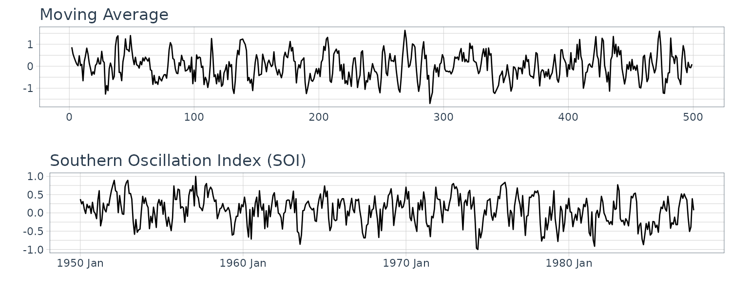     

Autoregressions

To generate a somewhat periodic behavior, we can turn to autoregression model. For example:

\[\begin{aligned} x_{t} &= x_{t-1} - 0.9x_{t-2} + w_{t} \end{aligned}\]

We can see the resemblance to the speech data:

dat$x <- stats::filter(dat$w, filter = c(1, -0.9), method = "recursive")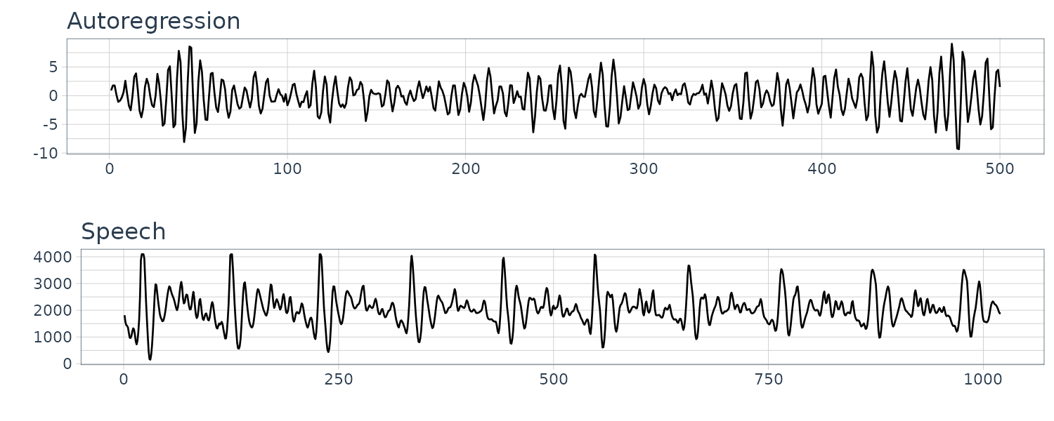     

Random Walk with Drift

\[\begin{aligned} x_{t} &= \delta + x_{t-1} + w_{t}\\ x_{0} &= 0 \end{aligned}\]

The above is the same as a cumulative sum of white noise variates:

\[\begin{aligned} x_{t} &= \delta t + \sum_{j=1}^{t}w_{j} \end{aligned}\]

And the mean:

\[\begin{aligned} \mu_{xt} &= E[x_{t}]\\ &= \delta t + \sum_{j=1}^{t}E[w_{j}]\\ &= \delta t \end{aligned}\]

autocovariance function:

\[\begin{aligned} \gamma_{x}(s, t) &= \mathrm{cov}(x_{s}, x_{t})\\ &= \mathrm{cov}\Big( \sum_{j=1}^{s}w_{j}, \sum_{k = 1}^{t}w_{k} \Big)\\ &= \mathrm{min}\{s, t\}\sigma_{w}^{2} \end{aligned}\]

Because \(w_{t}\) are uncorrelated, and thus only the overlapped variances are added. Note that the autocovariance function depends on particular values of \(s\) and \(t\), and thus not stationary.

For the variance:

\[\begin{aligned} \mathrm{var}(x_{t}) &= \gamma_{x}(t, t)\\ &= t\sigma_{w}^{2} \end{aligned}\]

Note that the variance increases without bound as time \(t\) increases.

And note the resemblance to Global Temperature Deviations:

dat$xd <- cumsum(dat$w + 0.2)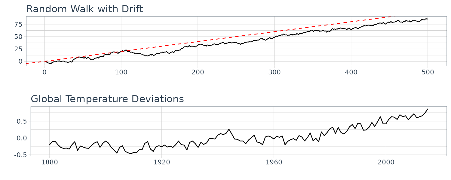     

Trend Stationarity

Consider the model:

\[\begin{aligned} x_{t} &= \alpha + \beta t + y_{t} \end{aligned}\]

Where \(y_{t}\) is stationary. Then the mean:

\[\begin{aligned} \mu_{x, t} &= E[x_{t}]\\ &= \alpha + \beta t + \mu_{y} \end{aligned}\]

Which is not independent of time. However, for the autocovariance function:

\[\begin{aligned} \gamma_{x}(h) &= \mathrm{cov}(x_{t+h}, x_{t})\\ &= E[(x_{t+h} - \mu_{x, t+h})(x_{t} - \mu_{x,t})]\\ &= E[(y_{t+h} - \mu_{y})(y_{t} - \mu_{y})]\\ &= \gamma_{y}(h) \end{aligned}\]

Is independent of time. In other words, after removing the trend, the model is staionary, or the model is considered stationary around a linear trend.

Signal in Noise

Consider the model:

\[\begin{aligned} x_{t} &= 2 \mathrm{cos}(2\pi \frac{t + 15}{50}) + w_{t} \end{aligned}\]

And the mean:

\[\begin{aligned} \mu_{xt} &= E[x_{t}]\\ &= E\Big[2\mathrm{cos}(2\pi \frac{t+15}{50}) + w_{t}\Big]\\ &= 2\mathrm{cos}(2\pi \frac{t+15}{50}) + E[w_{t}]\\ &= 2\mathrm{cos}(2\pi \frac{t+15}{50}) \end{aligned}\]

Note that any sinusoidal wave can be written as:

\[\begin{aligned} A \mathrm{cos}(2\pi \omega t + \phi) \end{aligned}\]

In the example:

\[\begin{aligned} A &= 2\\ \omega &= \frac{1}{50}\\ \phi &= \frac{2\pi 15}{50}\\ &= 0.6 \pi \end{aligned}\]

Adding white noise to the signal:

w <- rnorm(500, 0, 1)
cs <- 2 * cos(2 * pi * 1:500 / 50 + .6 * pi)      
dat <- tsibble(
  t = 1:500,
  cs = cs + w,
  index = t
)

Note the similarity with fMRI series:

Classical Regression

In a classical linear regression model:

\[\begin{aligned} x_{t} &= \beta_{0} + \beta_{1}z_{t1} + \cdots + \beta_{q}z_{tq} + w_{t} \end{aligned}\]

For time series regression, it is rarely the case where the residual is white noise.

For example, consider the monthly price (per pound) of a chicken for 180 months:

chicken <- as_tsibble(chicken)
chicken <- tsibble(
  t = 1:nrow(chicken),
  value = chicken$value,
  index = t
)
> chicken
# A tsibble: 180 x 2 [1]
       t value
   <int> <dbl>
 1     1  65.6
 2     2  66.5
 3     3  65.7
 4     4  64.3
 5     5  63.2
 6     6  62.9
 7     7  62.9
 8     8  62.7
 9     9  62.5
10    10  63.4
# ℹ 170 more rows
# ℹ Use `print(n = ...)` to see more rows      

Linear regression model:

\[\begin{aligned} x_{t} &= \beta_{0} + \beta_{1}z_{t} + w_{t} \end{aligned}\]

We would like to minimize the SSE:

\[\begin{aligned} \text{SSE} &= \sum_{t = 1}^{n}(x_{t} - \Big(\beta_{0} + \beta_{1}z_{t})^{2}\Big) \end{aligned}\]

By differentiating and setting both parameters to 0, we get:

\[\begin{aligned} \hat{\beta_{1}} &= \frac{\sum_{t=1}^{n}(x_{t} - \bar{x})(z_{t} - \bar{z})}{\sum_{t=1}^{n}(z_{t} - \bar{z})}\\ \hat{\beta}_{0} &= \bar{x} - \hat{\beta}_{1}\bar{z} \end{aligned}\]

Using R to fit a linear model:

fit <- lm(value ~ t, data = chicken)

chicken |>
  autoplot(value) +
  geom_abline(intercept = coef(fit)[1], slope = coef(fit)[2], col = "red") +      
  xlab("") +
  ylab("") +
  ggtitle("Chicken Prices") +
  theme_tq()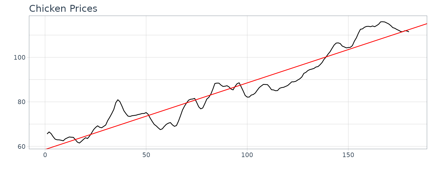

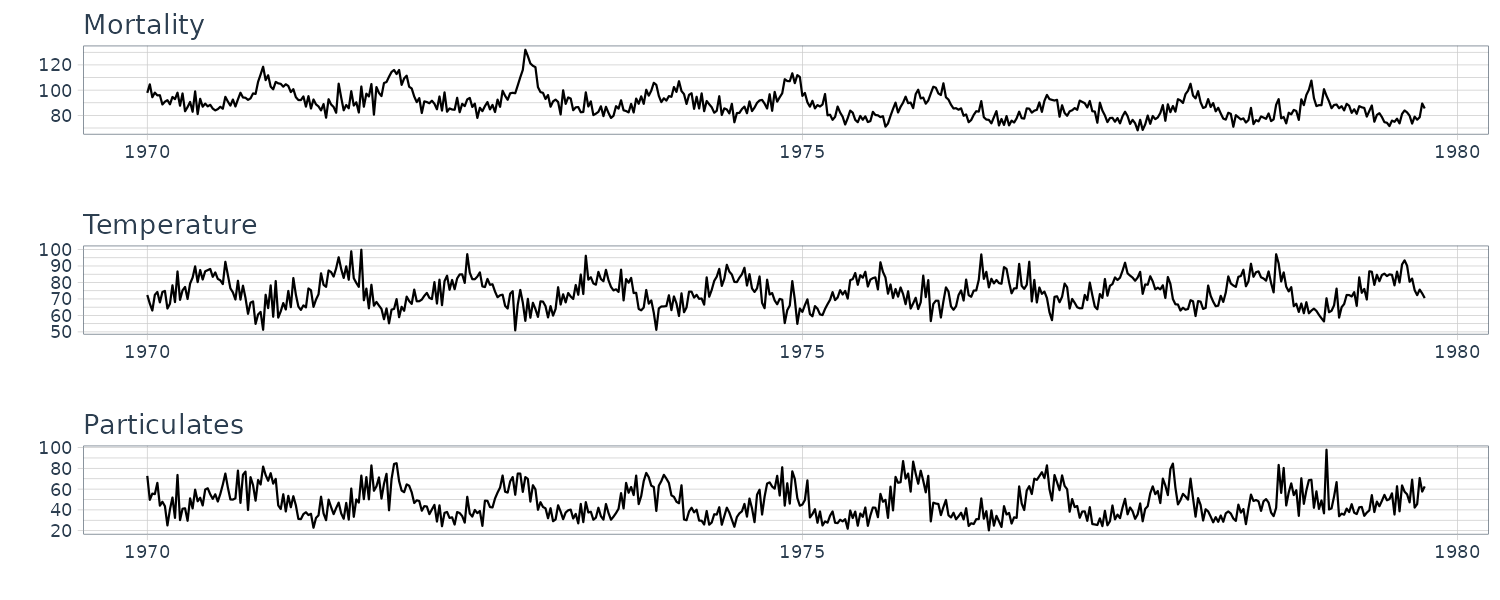
Example: Pollution, Temperature and Mortality

Let’s take a look at another example where we have more than one explanatory variables. We look at the possible effects of temperature and pollution on weekly mortality in LA county.

Taking a look at the time plots, we can see strong seasonal components in all 3 series:

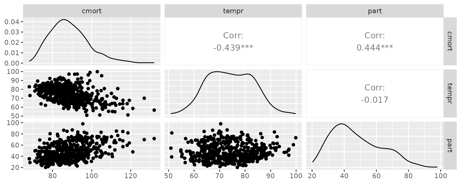
From the scatterplot, we can see strong linear relations between mortality and temperature and also pollutant. The mortality vs pollutants indicate a possible quadratic shape:

GGally::ggpairs(     
  dat,
  columns = 2:4
)

We will attempt to fit the following models:

\[\begin{aligned} M_{t} &= \beta_{0} + \beta_{1}t + w_{t}\\ M_{t} &= \beta_{0} + \beta_{1}t + \beta_{2}(T_{t} - T_{\mu}) + w_{t}\\ M_{t} &= \beta_{0} + \beta_{1}t + \beta_{2}(T_{t} - T_{\mu}) + \beta_{3}(T_{3} - T_{\mu})^{2} + w_{t}\\ M_{t} &= \beta_{0} + \beta_{1}t + \beta_{2}(T_{t} - T_{\mu}) + \beta_{3}(T_{3} - T_{\mu})^{2} + \beta_{4}P_{4} + w_{t}\\ \end{aligned}\]

Fitting the models in R:

fit1 <- lm(cmort ~ trend, data = dat)
fit2 <- lm(cmort ~ trend + temp, data = dat)
fit3 <- lm(cmort ~ trend + temp + temp2, data = dat)
fit4 <- lm(cmort ~ trend + temp + temp2 + part, data = dat)     

> anova(fit1, fit2, fit3, fit4)
Analysis of Variance Table

Model 1: cmort ~ trend
Model 2: cmort ~ trend + temp
Model 3: cmort ~ trend + temp + temp2
Model 4: cmort ~ trend + temp + temp2 + part
  Res.Df   RSS Df Sum of Sq       F    Pr(>F)    
1    506 40020                                   
2    505 31413  1    8606.6 211.090 < 2.2e-16 ***
3    504 27985  1    3428.7  84.094 < 2.2e-16 ***
4    503 20508  1    7476.1 183.362 < 2.2e-16 ***

We can see each subsequent model does better via the RSS/SSE.

Example: Regression With Lagged Variables

We saw the the Southern Oscillation Index (SOI) with a lag of 6 months is highly correlated with the Recruitment series. We therefore consider the following model:

\[\begin{aligned} R_{t} &= \beta_{0} + \beta_{1}S_{t-6} + w_{t} \end{aligned}\]

Fitting the model in R:

dat <- tsibble(
  t = rec$index,
  soiL6 = lag(soi$value, 6),
  rec = rec$value,
  index = t
)

fit <- lm(rec ~ soiL6, data = dat)     
> summary(fit)
Call:
lm(formula = rec ~ soiL6, data = dat)

Residuals:
    Min      1Q  Median      3Q     Max 
-65.187 -18.234   0.354  16.580  55.790 

Coefficients:
            Estimate Std. Error t value Pr(>|t|)    
(Intercept)   65.790      1.088   60.47   <2e-16 ***
soiL6        -44.283      2.781  -15.92   <2e-16 ***
---
Signif. codes:  0 ‘***’ 0.001 ‘**’ 0.01 ‘*’ 0.05 ‘.’ 0.1 ‘ ’ 1

Residual standard error: 22.5 on 445 degrees of freedom
  (6 observations deleted due to missingness)
Multiple R-squared:  0.3629,	Adjusted R-squared:  0.3615        
F-statistic: 253.5 on 1 and 445 DF,  p-value: < 2.2e-16

The fitted model is:

\[\begin{aligned} \hat{R}_{t} &= 65.79 - 44.28S_{t-6} \end{aligned}\]

Exploratory Data Analysis

Trend Stationarity

The easiest form of nonstationarity to work with is trend stationary model:

\[\begin{aligned} x_{t} &= \mu_{t} + y_{t} \end{aligned}\]

Where \(\mu_{t}\) is the trend and \(y_{t}\) is a stationary process. We will work with the detrended residual:

\[\begin{aligned} \hat{y}_{t} &= x_{t} - \hat{\mu}_{t} \end{aligned}\]

Example: Detrending Chicken Prices

Recall the model for the chicken prices:

> summary(fit)

Call:
lm(formula = value ~ t, data = chicken)

Residuals:
    Min      1Q  Median      3Q     Max 
-8.7411 -3.4730  0.8251  2.7738 11.5804 

Coefficients:
             Estimate Std. Error t value Pr(>|t|)    
(Intercept) 58.583235   0.703020   83.33   <2e-16 ***
t            0.299342   0.006737   44.43   <2e-16 ***
---
Signif. codes:  0 ‘***’ 0.001 ‘**’ 0.01 ‘*’ 0.05 ‘.’ 0.1 ‘ ’ 1       

Residual standard error: 4.696 on 178 degrees of freedom
Multiple R-squared:  0.9173,	Adjusted R-squared:  0.9168      
F-statistic:  1974 on 1 and 178 DF,  p-value: < 2.2e-16

\[\begin{aligned} \hat{\mu}_{t} &= 59 + 0.30 t \end{aligned}\]

To obtain the detrended series:

\[\begin{aligned} \hat{y}_{t} &= x_{t} - 59 - 0.30 t \end{aligned}\]

The plot:

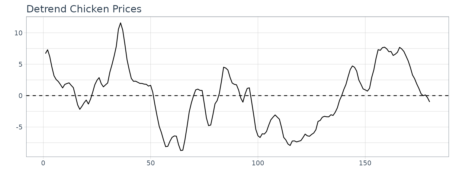
The ACF plot:

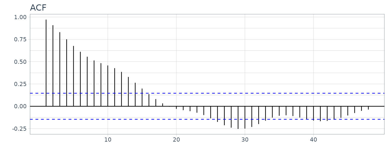
It is also possible to treat the model as a random walk with drift model:

\[\begin{aligned} \mu_{t} &= \delta + \mu_{t-1} + w_{t} \end{aligned}\]

Differencing the data will yield a stationary process:

\[\begin{aligned} \mu_{t} - \mu_{t-1} &= \delta + w_{t}\\ x_{t} - x_{t-1} &= (\mu_{t} + y_{t}) - (\mu_{t-1} + y_{t-1})\\ &= (\mu_{t} - \mu_{t-1}) + (y_{t} - y_{t-1})\\ \delta &= \mu_{t} - \mu_{t-1}\\ w_{t} &= y_{t} - y_{t-1} \end{aligned}\]

One disadvantage of differencing is it does not yield an estimate for the stationary process \(y_{t}\).

Differencing (Backshift Operator)

We define the backshift operator as:

\[\begin{aligned} Bx_{t} &= x_{t-1}\\ B^{2}x_{t} &= B(Bx_{t})\\ &= B(x_{t-1})\\ &= x_{t-2}\\ B^{k} &= x_{t-k} \end{aligned}\]

We also require that:

\[\begin{aligned} B^{-1}B &= 1 x_{t} &= B^{-1}Bx_{t}\\ &= B^{-1}x_{t-1} \end{aligned}\]

\(B^{-1}\) is known as the forward-shift operator.

We denote the first difference as:

\[\begin{aligned} \nabla x_{t} &= x_{t} - x_{t-1}\\ &= (1 - B)x_{t} \end{aligned}\]

And second order difference:

\[\begin{aligned} \nabla^{2}x_{t} &= (1 - B)^{2}x_{t}\\ &= (1 - 2B + B^{2})x_{t}\\ &= x_{t} - 2x_{t-1} + x_{t-2}\\[5pt] \nabla(\nabla x_{t}) &= \nabla(x_{t} - x_{t-1})\\ &= (x_{t} - x_{t-1}) - (x_{t-1} - x_{t-2})\\ &= x_{t} - 2x_{t-1} + x_{t-2} \end{aligned}\]

In general, differences of order d are defined as:

\[\begin{aligned} \nabla^{d} &= (1 - B)^{d} \end{aligned}\]

Transformation

Sometimes transformations may be useful to equalize the variability of a time series. One example of such transformation is the log transform:

\[\begin{aligned} y_{t} &= \mathrm{log}(x_{t}) \end{aligned}\]

Power transformations in the Box-Cox family are of the form:

\[\begin{aligned} y_{t} &= \begin{cases} \frac{x_{t}^{\lambda} - 1}{\lambda} & \lambda \neq 0\\ \mathrm{log}(x_{t}) & \lambda = 0 \end{cases} \end{aligned}\]

Transformations are normally done to improve linearity and normality.

Lagged Scatterplot Matrix

The ACF gives a linear correlation of lags. However, the relationship might be nonlinear. The example in this section displays the lagged scatterplot of the SOI series. Lowess (locally weighted scatterplot smoothing) are plotted together with the scatterplot to help show the nonlinear relationship.

library(astsa)
lag1.plot(as.ts(soi), 12)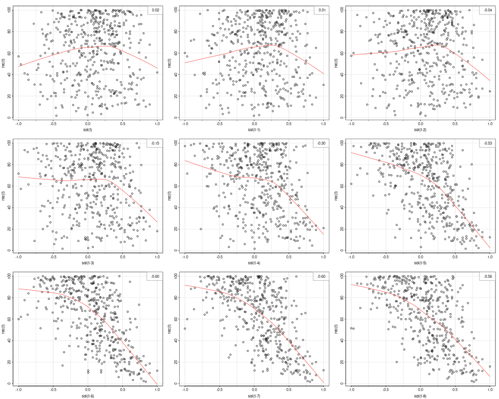     

We can see the correlation is highest at t-6. However the relationship is nonlinear. In this case, we could add a dummy variable to implement a segmented regression (hockey stick):

\[\begin{aligned} R_{t} &= \beta_{0} + \beta_{1}S_{t-6} + \beta_{2}D_{t-6} + \beta_{3}D_{t-6} + w_{t}\\[5pt] R_{t} &= \begin{cases} \beta_{0} + \beta_{1}S_{t-6} + w_{t} & S_{t-6} < 0\\ (\beta_{0} + \beta_{2}) + (\beta_{1} + \beta_{3})S_{t-6} + w_{t} & S_{t-6} \geq 0 \end{cases} \end{aligned}\]

dummy <- ifelse(soi$value < 0, 0, 1)

dat <- tibble(
  rec = rec$value,
  soi = soi$value,
  soiL6 = lag(soi, 6),
  dL6 = lag(dummy, 6)
) |>
  mutate(
    lowessx = c(rep(NA, 6), lowess(soiL6[7:n()], rec[7:n()])$x),      
    lowessy = c(rep(NA, 6), lowess(soiL6[7:n()], rec[7:n()])$y)
  )

fit <- lm(rec ~ soiL6 * dL6, data = dat)
> summary(fit)
Call:
lm(formula = rec ~ soiL6 * dL6, data = dat)

Residuals:
    Min      1Q  Median      3Q     Max 
-63.291 -15.821   2.224  15.791  61.788 

Coefficients:
            Estimate Std. Error t value             Pr(>|t|)    
(Intercept)   74.479      2.865  25.998 < 0.0000000000000002 ***
soiL6        -15.358      7.401  -2.075               0.0386 *  
dL6           -1.139      3.711  -0.307               0.7590    
soiL6:dL6    -51.244      9.523  -5.381           0.00000012 ***
---
Signif. codes:  0 ‘***’ 0.001 ‘**’ 0.01 ‘*’ 0.05 ‘.’ 0.1 ‘ ’ 1

Residual standard error: 21.84 on 443 degrees of freedom
  (6 observations deleted due to missingness)
Multiple R-squared:  0.4024,	Adjusted R-squared:  0.3984 
F-statistic: 99.43 on 3 and 443 DF,  p-value: < 0.00000000000000022         

Plotting the lowess and fitted curve:

dat$fitted <- c(rep(NA, 6), fitted(fit))
dat |>
  ggplot(aes(x = soiL6, y = rec)) +
  geom_point() +
  geom_line(aes(y = lowessy, x = lowessx), col = "blue") +     
  geom_line(aes(y = fitted), col = "red") +
  ggtitle("Rec vs SOIL6")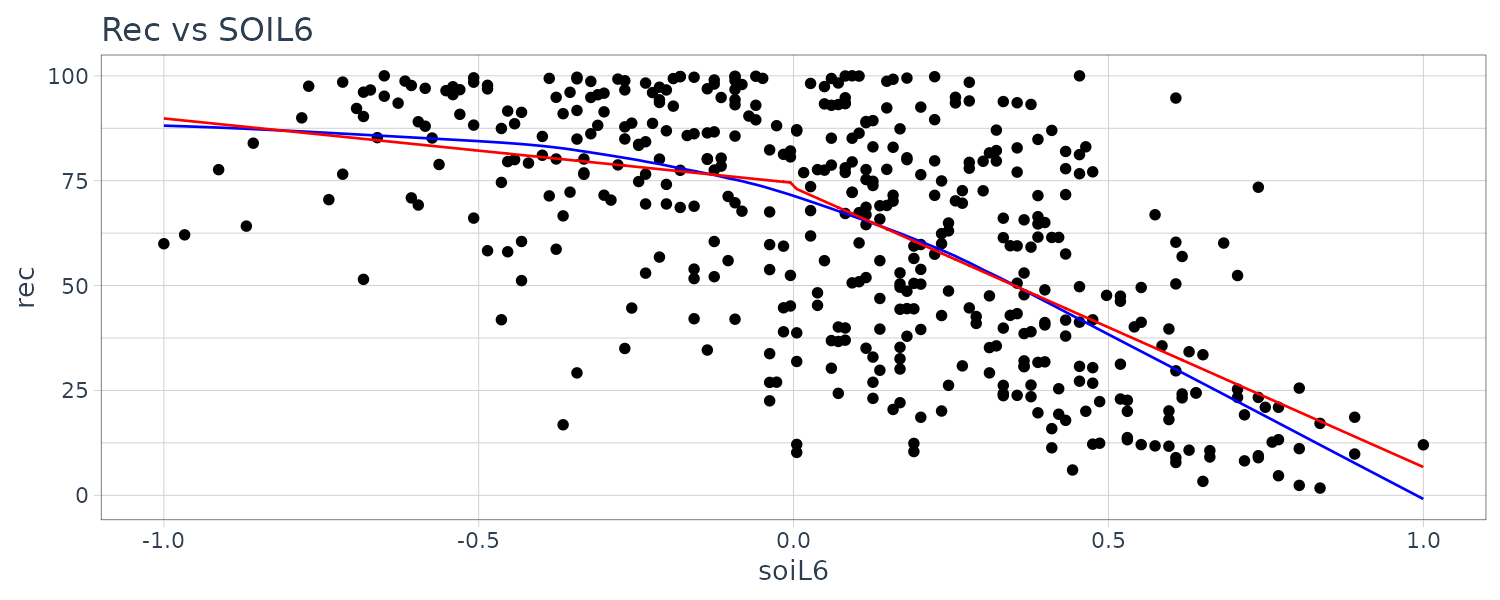

Smoothing

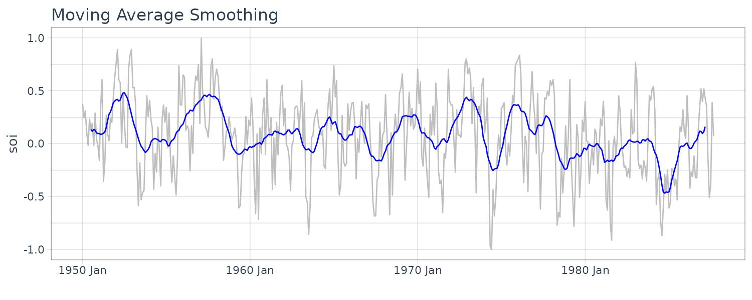
Moving Average Smoothing

If \(x_{t}\) represents the data observations, then:

\[\begin{aligned} m_{t} &= \sum_{j= -k}^{k}a_{j}x_{t-j}\\ a_j &= a_{-j} \geq 0 \end{aligned}\] \[\begin{aligned} \sum_{j=-k}^{k}a_{j} &= 1 \end{aligned}\]

For example, using the monthly SOI series for \(k = 6\) using weights:

\[\begin{aligned} a_{0} &= a_{\pm 1} = \cdots = a_{\pm 5} = \frac{1}{12} \end{aligned}\] \[\begin{aligned} a_{\pm 6} &= \frac{1}{24} \end{aligned}\]

weights <- c(.5, rep(1, 11), .5) / 12
dat <- tsibble(
  t = soi$index,
  soi = soi$value,
  smth = stats::filter(soi, sides = 2, filter = weights),      
  index = t
)

Kernel Smoothing

Although the moving average smoothing highlight the EL Nino effect, the smoothing still look too choppy. We can obtain a smoother fit using normal distribution for the weights (kernel smoothing) rather than the boxcar-type weights above. “b” is the bandwidth and \(K()\) is known as the kernel function.

\[\begin{aligned} m_{t} &= \sum_{i=1}^{n}w_{i}(t)x_{i}\\ w_{i}(t) &= \frac{K\Big(\frac{t-i}{b}\Big)}{\sum_{j=1}^{n}K\Big(\frac{t-i}{b}\Big)} \end{aligned}\] \[\begin{aligned} K(z) &= \frac{1}{\sqrt{2\pi}}e^{\frac{-z^{2}}{2}} \end{aligned}\]

To implement this in R, we use the “ksmooth” function. The wider the bandwidth, the smoother the result. In the SOI example, we use a value of \(b=12\) to corespond to approximately smoothing a little over a year.

dat$ksmooth <- ksmooth(    
  time(soi$index),
  soi$value,
  "normal",
  bandwidth = 12
)$y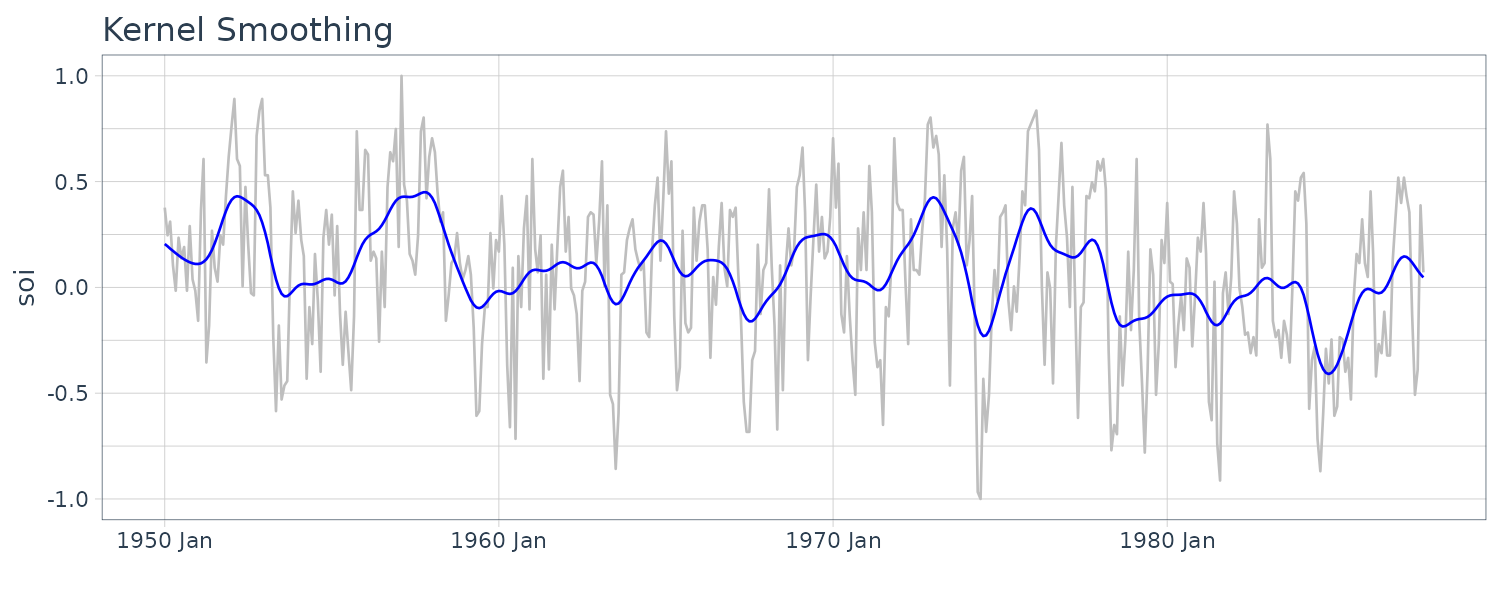

Lowess

Lowest is a method of smoothing that employs nearest neighbor local regression. The larger the fraction of nearest neighbors are included, the smoother the fit will be. We fit 2 lowess curve where one is smoother than the other:

dat$lowess1 <- lowess(soi$value, f = 0.05)$y    
dat$lowess2 <- lowess(soi$value)$y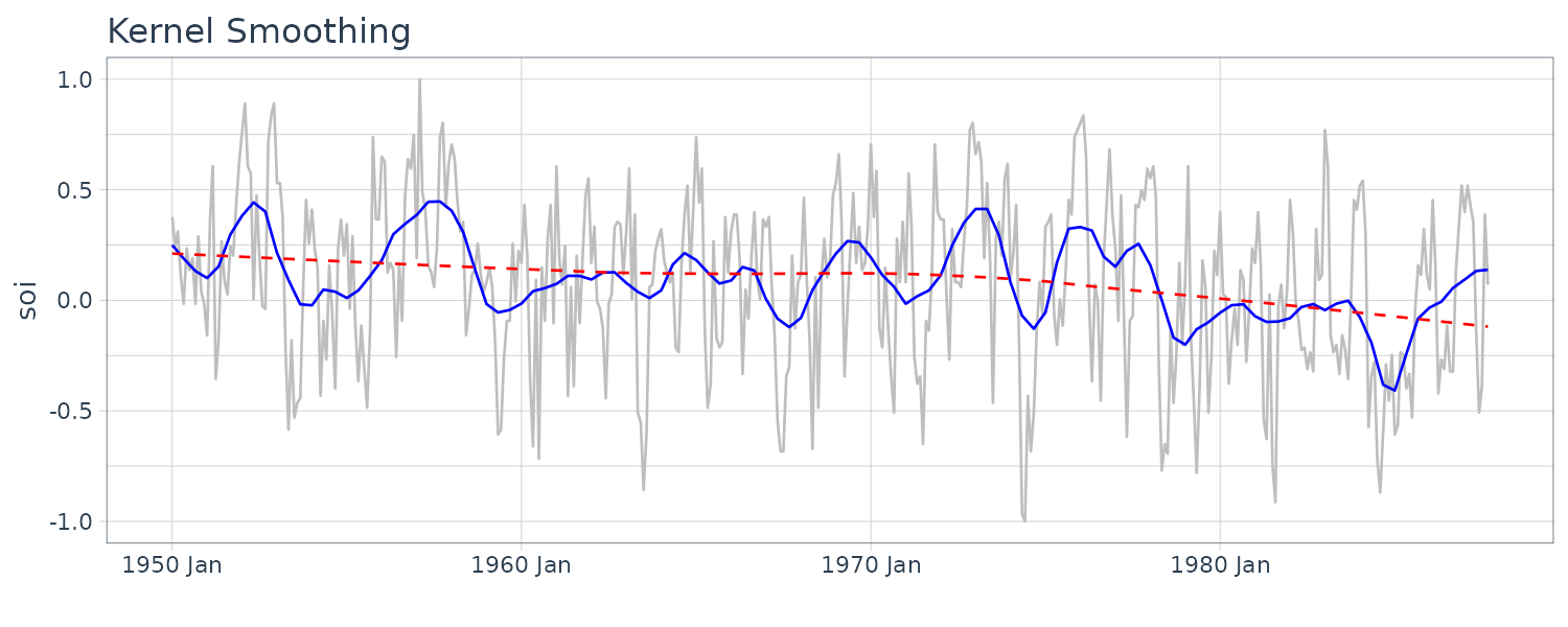

Smoothing Splines

Given a cubic polynomial:

\[\begin{aligned} m_{t} &= \beta_{0} + \beta_{1}t + \beta_{2}t^{2} + \beta_{3}t^{3} \end{aligned}\]

Cubic splines divide the time into \(k\) intervals. The values \(t_{0}, t_{1}, \cdots, t_{k}\) are called knots. In each interval, a cublic polynomial is fit with conditions that the ends are connected.

For smoothing splines, the following objective function is minimized given a regularizing \(\lambda > 0\):

\[\begin{aligned} \sum_{t=1}^{n}(x_{t} - m_{t})^{2} + \lambda \int (m_{t}^{\prime\prime})^{2}\ dt \end{aligned}\]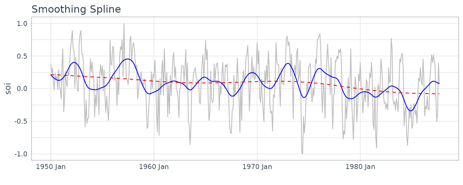

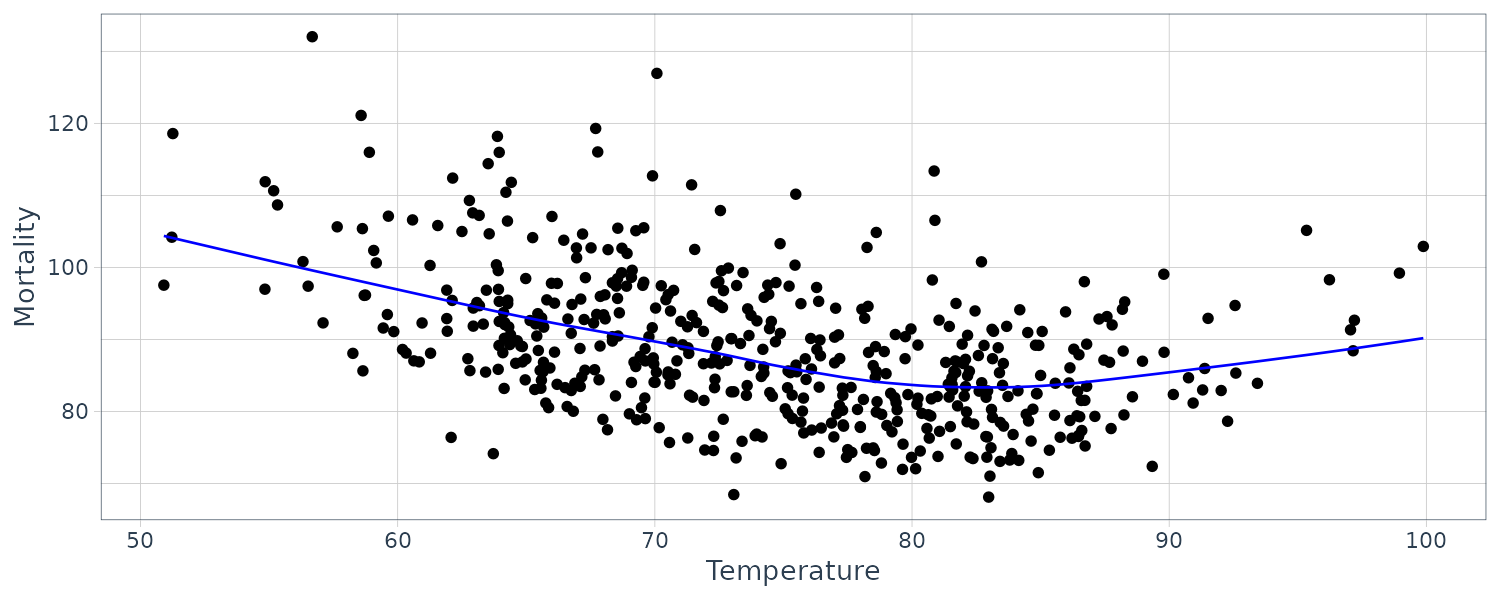
2D Smoothing

It is also possible to smooth one series over another. Using the Temperature and Mortality series data:

dat <- tibble(
  tempr = tempr$value,
  cmort = cmort$value,
  lowess_y = lowess(tempr, cmort)$y,     
  lowess_x = lowess(tempr, cmort)$x
)

ARIMA

AR Model

An AR(p) is of the form:

\[\begin{aligned} x_{t} &= \phi_{1}x_{t-1} + \phi_{2}x_{t-2} + \cdots + \phi_{p}x_{t-p} + w_{t} \end{aligned}\]

Where \(x_{t}\) is stationary. If the mean of \(x_{t}\) is not zero:

\[\begin{aligned} x_{t} - \mu &= \phi_{1}(x_{t-1} - \mu) + (\phi_{2}x_{t-2} - \mu) + \cdots + (\phi_{p}x_{t-p} - \mu) + w_{t}\\ x_{t} &= \alpha + \phi_{1}x_{t-1} + \phi_{2}x_{t-2} + \cdots + \phi_{p}x_{t-p} + w_{t}\\ \alpha &= \mu(1 - \phi_{1} - \cdots - \phi_{p}) \end{aligned}\]

We can simply the notation using the backshift operator:

\[\begin{aligned} (1 - \phi_{1}B - \phi_{2}B^{2} - \cdots - \phi_{p}B^{p})x_{t} &= w_{t}\\ \phi(B)x_{t} &= w_{t} \end{aligned}\]

\(\phi(B)\) is known as the autoregressive operator.

For example, for a AR(1) model:

\[\begin{aligned} x_{t} &= \phi x_{t-1} + w_{t}\\ \phi(\phi x_{t-2} + w_{t-1}) + w_{t}\\ \vdots\\ &= \phi^{k}x_{t - k} + \sum_{j=0}^{k-1}\phi^{j}w_{t-j} \end{aligned}\]

Suppose that \(\mid \phi \mid < 1\) and the variance is finite:

\[\begin{aligned} x_{t} &= \sum_{j= 0}^{\infty}\phi^{j}w_{t-j} \end{aligned}\]

And stationary with mean:

\[\begin{aligned} E[x_{t}] &= \sum_{j=0}^{\infty}\phi^{j}E[w_{t-j}]\\ &= 0 \end{aligned}\]

And the autocovariance function for a stationary AR(1) model:

\[\begin{aligned} \gamma(h) &= \text{cov}(x_{t+h}, x)\\ &= E\Bigg[\Big(\sum_{j=0}^{\infty}\phi^{j}w_{t+h - j}\Big) \Big(\sum_{k=0}^{\infty}\phi^{k}w_{t+h - k}\Big)\Bigg]\\ &= E[(w_{t+h} + \cdots + \phi^{h}w_{t} + \phi^{h+1}w_{t-1} + \cdots)(w_{t} + \phi w_{t-1} + \cdots)]\\ &= E[w_{t}^{2}]\sum_{j=0}^{\infty}\phi^{j+j}\phi^{j}\\ &= \sigma_{w}^{2}\sum_{j = 0}^{\infty}\phi^{h+j}\phi^{j}\\ &= \sigma_{w}^{2}\phi^{h}\sum_{j=0}^{\infty}\phi^{2j}\\ &= \sigma_{w}\frac{\phi^{h}}{1 - \phi^{2}}\\ h &\geq 0 \end{aligned}\]

We only look at \(h \geq 0\) because:

\[\begin{aligned} \gamma(h) = \gamma(-h) \end{aligned}\]

The ACF of AR(1):

\[\begin{aligned} \rho(h) &= \frac{\gamma(h)}{\gamma(0)}\\ &= \frac{\sigma_{w}\frac{\phi^{h}}{1 - \phi^{2}}}{\sigma_{w}\frac{\phi^{0}}{1 - \phi^{2}}}\\ &= \phi^{h} \end{aligned}\]

And \(\rho(h)\) satisfies the recursion:

\[\begin{aligned} \rho(h) &= \phi \rho(h - 1) \end{aligned}\]

Let’s simulate two time series with \(\phi = 0.9\) and \(\phi = -0.9\):

dat1 <- as_tsibble(
  arima.sim(
    list(order = c(1, 0, 0), ar = 0.9),
    n = 100
  )
)
dat2 <- as_tsibble(
  arima.sim(
    list(order = c(1, 0, 0), ar = -0.9),      
    n = 100
  )
)

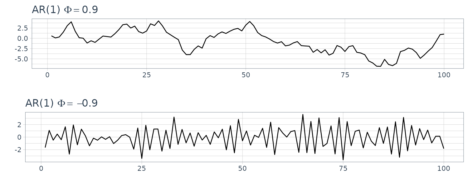
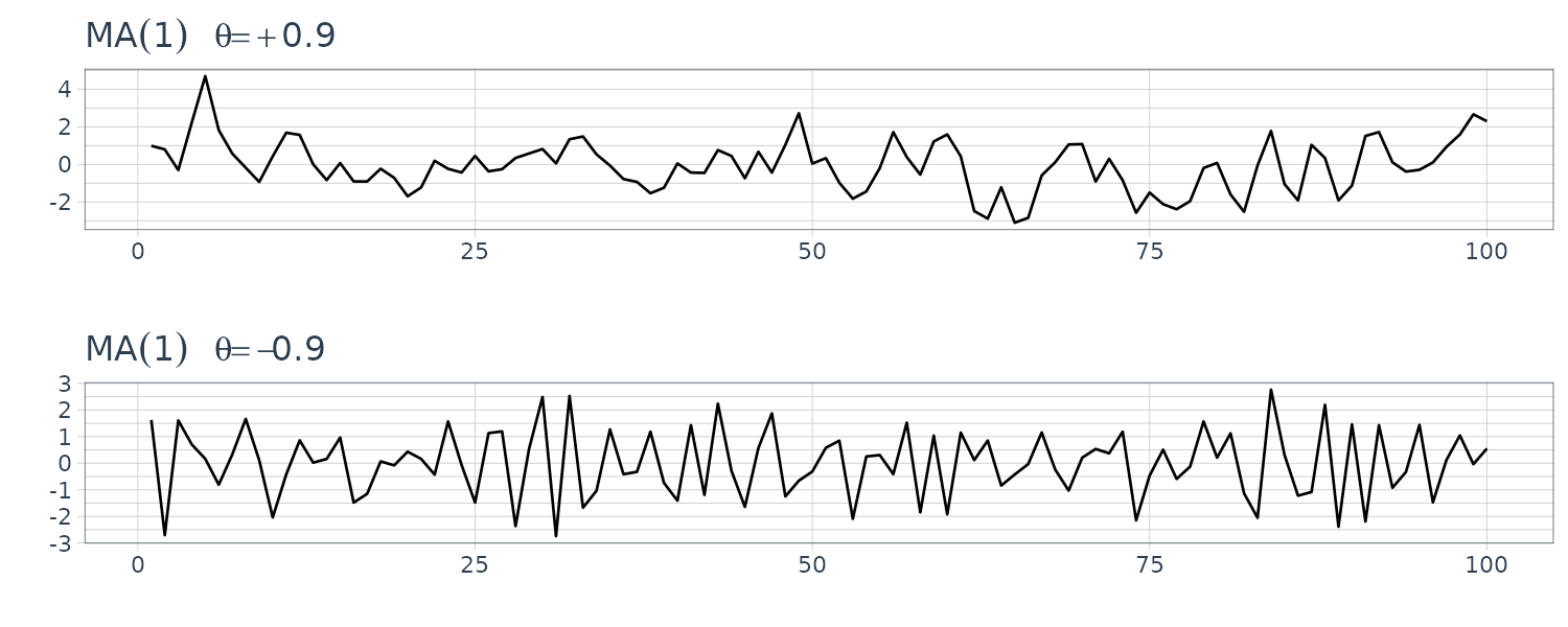
\(\phi = -0.9\) appears choppy because the points are negatively correlated. When one point is positive, the next point is likely to be negative.

Consider the AR(1) in operator form:

\[\begin{aligned} \phi(B)x_{t} &= w_{t}\\ \phi(B) &= 1 - \phi B\\ |\phi| &< 1 \end{aligned}\] \[\begin{aligned} x_{t} &= \sum_{j=0}^{\infty}\psi_{j}w_{t-j}\\ &= \psi(B)w_{t}\\ \psi_{j} &= \phi^{j} \end{aligned}\]

Suppose we do not know \(\phi_{j} = \phi^{j}\). We know that:

\[\begin{aligned} \phi(B)x_{t} &= w_{t} \end{aligned}\]

Substituting \(x_{t} = \psi(B)w_{t}\):

\[\begin{aligned} \phi(B)\psi(B)w_{t} &= w_{t} \end{aligned}\] \[\begin{aligned} (1 - \phi B)(1 + \psi_{1}B + \psi_{2}B^{2} + \cdots + \psi_{j}B^{j} + \cdots) &= 1\\ 1 + (\psi_{1} - \phi)B + (\psi_{2} - \psi_{1}\phi)B^{2} + \cdots + (\psi_{j} - \psi_{j-1}\phi)B^{j} + \cdots &= 1 \end{aligned}\]

Hence, all the cofficients of B have to be 0:

\[\begin{aligned} \psi_{1} - \phi &= 0\\ \psi_{2} - \psi_{1}\phi &= 0\\ \vdots\\ \psi_{j} &= \psi_{j-1}\phi \end{aligned}\]

Another way to represent this is to assume an inverse operator exist:

\[\begin{aligned} \phi^{-1}(B)\phi(B)x_{t} &= \phi^{-1}(B)w_{t}\\ x_{t} &= \phi^{-1}(B)w_{t} \end{aligned}\]

We already know that:

\[\begin{aligned} \phi^{-1}(B) &= 1 + \psi_{1}B + \psi_{2}B^{2} + \cdots + \psi_{j}B^{j} + \cdots \end{aligned}\]

We can treat the B operator as a complex number z:

\[\begin{aligned} \phi^{-1}(z) &= \frac{1}{1 - \phi z}\\ &= 1 + \phi z + \phi^{2}z^{2} + \cdots + \phi^{j}z^{z} + \cdots\\ |z| &\leq 1 \end{aligned}\]

MA Models

The MA(q) model is defined as:

\[\begin{aligned} x_{t} &= w_{t} + \theta_{1}w_{t-1} + \theta_{2}w_{t-2} + \cdots + \theta_{q}w_{t-q} \end{aligned}\] \[\begin{aligned} x_{t} &= \theta(B)w_{t} \end{aligned}\] \[\begin{aligned} \theta(B) &= 1 + \theta_{1}B + \theta_{2}B^{2} + \cdots + \theta_{q}B^{q} \end{aligned}\]

Consider the MA(1) model:

\[\begin{aligned} x_{t} &= w_{t} + \theta w_{t-1} \end{aligned}\]

The autocovariance function:

\[\begin{aligned} \gamma(h) &= \begin{cases} (1 + \theta^{2})\sigma_{w}^{2} & h = 0\\ \theta \sigma_{w}^{2} & h = 1\\ 0 & h > 1 \end{cases} \end{aligned}\]

ACF:

\[\begin{aligned} \rho(h) &= \begin{cases} \frac{\theta}{1 + \theta^{2}} & h = 1\\ 0 & h > 1 \end{cases} \end{aligned}\]

In other words, \(x_{t}\) is only correlated with \(x_{t-1}\). This is unlike AR(1) model where the autocorrelation is never 0.

Simulating MA(1) models:

dat1 <- as_tsibble(
  arima.sim(
    list(order = c(0, 0, 1), ma = 0.9),
    n = 100
  )
)

dat2 <- as_tsibble(
  arima.sim(
    list(order = c(0, 0, 1), ma = -0.9),      
    n = 100
  )
)

To convert the MA(1) to an infinite AR representation, we can do the recursive subsitution:

\[\begin{aligned} w_{t} &= -\theta w_{t-1} + x_{t}\\ &= -\theta(-\theta w_{t-2} + x_{t-1}) + x_{t}\\ &= \theta^{2} w_{t-2} + \theta x_{t-1} + x_{t}\\ \vdots\\ &= \sum_{j=0}^{\infty}(-\theta)^{j}x_{t-j}\\ |\theta| &< 1 \end{aligned}\]

ARMA Models

A time series is ARMA(p, q) if it is stationary and:

\[\begin{aligned} x_{t} &= \phi_{1}x_{t-1} + \cdots + \phi_{p}x_{t-p} + w_{t} + \theta_{1}w_{t-1} + \cdots + \theta_{q}w_{t-q} \end{aligned}\]

If \(x_{t}\) has a nonzero mean, we set:

\[\begin{aligned} \alpha &= \mu(1 - \phi_{1} - \cdots - \phi_{p})\\ x_{t} &= \alpha + \phi_{1}x_{t-1} + \cdots + \phi_{p}x_{t-p} + w_{t} + \theta_{1}w_{t-1} + \cdots + \theta_{q}w_{t-q} \end{aligned}\]

ARMA(p, q) can be written in a more concise form:

\[\begin{aligned} \phi(B)x_{t} &= \theta(B)w_{t} \end{aligned}\]

There are 3 main problems when it comes to ARMA(p, q) models.

1) Parameter Redundant Models

To address this problem, we require \(\phi(z)\) and \(\theta(z)\) to have no common factors.

2) Stationary AR models that depend on the future

To address this problem, we require the model to be causal:

\[\begin{aligned} x_{t} &= \sum_{j=0}^{\infty}\psi_{j}w_{t-j}\\ &= \psi(B)w_{t}\\ \sum_{j=0}^{\infty}\psi_{j}w_{t-j}|\psi_{j}| &< \infty\\ \psi_{0} &= 1 \end{aligned}\]

For an ARMA(p, q) model:

\[\begin{aligned} \psi(z) &= \sum_{j=0}^{\infty}\psi_{j}z^{j}\\ &= \frac{\theta(z)}{\phi(z)} \end{aligned}\]

In order to be causal:

\[\begin{aligned} \phi(z) &\neq 0\\ |z| \leq 1 \end{aligned}\]

Another way to phrase the above is for the roots of \(\phi(z)\) to lie outside the unit circle:

\[\begin{aligned} \phi(z) &= 0\\ |z| > 1 \end{aligned}\]

In other words, having \(phi(z) = 0\) only when \(\mid z\mid > 1\).

3) MA models that are not unique

An ARMA(p, q) model is said to be invertible if:

\[\begin{aligned} \pi(B)x_{t} &= \sum_{j = 0}^{\infty}\pi_{j}x_{t-j}\\ &= w_{t}\\ \pi(B) &= \sum_{j=0}^{\infty}\pi_{j}B^{j}\\ \sum_{j=0}^{\infty}|\pi_{j}| &< \infty \end{aligned}\]

An ARIMA(p, q) model is invertible if and only if:

\[\begin{aligned} \pi(z) &= \sum_{j= 0}^{\infty}\pi_{j}z^{j}\\ &= \frac{\phi(z)}{\theta(z)}\\ \theta(z) \neq 0\\ |z| &\leq 1 \end{aligned}\]

In other words, an ARMA process is invertible only when the roots of \(\theta(z)\) lie outside the unit circle.

Let’s do an example. Consider the process:

\[\begin{aligned} x_{t} &= 0.4 x_{t-1} + 0.45x_{t-2} + w_{t} + w_{t-1} + 0.25w_{t-2}\\ \end{aligned}\] \[\begin{aligned} x_{t} - 0.4 x_{t-1} - 0.45x_{t-2} &= w_{t} + w_{t-1} + 0.25w_{t-2}\\ (1 - 0.4B - 0.45B^{2})x_{t} &= (1 + B + 0.25B^{2})w_{t}\\ (1 + 0.5B)(1 - 0.9B)x_{t} &= (1 + 0.5B)^{2}w_{t}\\ (1 - 0.9B)x_{t} &= (1 + 0.5B)w_{t}\\ \end{aligned}\] \[\begin{aligned} \phi(z) &= (1 - 0.9z)\\ \theta(z) &= (1 + 0.5z) x_{t} &= 0.9x_{t-1} + 0.5w_{t-1} + w_{t} \end{aligned}\]

The model is causal because:

\[\begin{aligned} \phi(z) &= (1 - 0.9z)\\ &= 0\\ z &= \frac{10}{9}\\ &> 0 \end{aligned}\]

And the model is invertible because:

\[\begin{aligned} \theta(z) &= (1 + 0.5z)\\ &= 0\\ z &= -1 \times 2\\ &= -2\\ |z| &> 1 \end{aligned}\]

Recall that:

\[\begin{aligned} \phi(z)\psi(z) &= \theta(z)\\ (1 - 0.9z)(1 + \psi_{1}z + \psi_{2}z^{2} + \cdots + \psi_{j}z^{j} + \cdots) &= 1 + 0.5z\\ 1 + (\psi_{1} - 0.9)z + (\psi_{2} - 0.9\psi_{1})z^{2} + \cdots + (\psi_{j} - 0.9\psi_{j-1})z^{j} + \cdots &= 1+0.5z\\ (\psi_{1} - 0.9)z &= 0.5z\\ \end{aligned}\]

For \(j = 1\):

\[\begin{aligned} \psi_{1} &= 0.5 + 0.9\\ &= 1.4\\ \end{aligned}\]

For \(j > 1\):

\[\begin{aligned} \psi_{j} - 0.9\psi_{j-1} &= 0\\ \psi_{j} &= 0.9\psi_{j-1} \end{aligned}\]

Thus:

\[\begin{aligned} \psi_{j} &= 1.4(0.9)^{j-1}\\ j &\geq 1\\ \psi_{0} &= 1\\ x_{t} &= \sum_{j = 0}^{\infty}\psi_{j}w_{t-j}\\ &= w_{t} + 1.4\sum_{j=1}^{\infty}0.9^{j-1}w_{t-j} \end{aligned}\]

We can get the values of \(\psi_{j}\) in R:

> ARMAtoMA(ar = 0.9, ma = 0.5, 10)
[1] 1.4000000 1.2600000 1.1340000 1.0206000 0.9185400        
[6 ]0.8266860 0.7440174 0.6696157 0.6026541 0.5423887

The invertible representation can be obtained by matching coefficients of:

\[\begin{aligned} \theta(z)\pi(z) &= \phi(z) \end{aligned}\] \[\begin{aligned} (1 + 0.5z)(1 + \pi_{1}z + \pi_{2}z^{2} + \cdots) &= 1 - 0.9z\\ 1 + (\pi_{1} + 0.5)z + (\pi_{2} + 0.5\pi_{1})z^{2} + \cdots + (\pi_{j} + 0.5\pi_{j-1})z^{j} + \cdots &= 1 - 0.9z \end{aligned}\] \[\begin{aligned} \pi_{1} + 0.5 &= -0.9\\ \pi_{1} &= -1.4\\ \pi_{2} + 0.5\pi_{1} &= 0\\ \pi_{2} &= -0.5 \times -1.4\\ \pi_{j} &= (-1)^{j}\sum_{j=1}^{\infty}(-0.5)^{j-1}x_{t-j} + w_{t} \end{aligned}\]

The values of \(\pi_{j}\) can be calculated in R by reversing the roles of \(w_{t}\) and \(x_{t}\):

\[\begin{aligned} w_{t} &= -0.5w_{t-1} + x_{t} - 0.9x_{t-1} \end{aligned}\]

> ARMAtoMA(ar = -0.5, ma = -0.9, 10)
[1] -1.400000000  0.700000000 -0.350000000  0.175000000 -0.087500000      
[6] 0.043750000 -0.021875000 0.010937500 -0.005468750  0.002734375

Causal Conditions AR(2)

For an AR(2) model to be causal, the two roots of \(\phi(z)\) has to lie outisde of the unit circle:

\[\begin{aligned} (1 - \phi_{1}B - \phi_{2}B^{2})x_{t} &= w_{t} \end{aligned}\] \[\begin{aligned} \phi(z) &= 1 = \phi_{1}z - \phi_{2}z^{2} \end{aligned}\]

The conditions must satisfied:

\[\begin{aligned} \Big|\frac{\phi_{1} \pm \sqrt{\phi_{1}^{2} + 4\phi_{2}}}{-2\phi_{2}} \Big| > 1 \end{aligned}\]

The roots could be real, equal, or complex conjugate pair. We can show that the following equivalent condition for causality:

\[\begin{aligned} \phi_{1} + \phi_{2} &< 1\\ \phi_{2} - \phi_{1} &< 1\\ |\phi_{2}| &< 1 \end{aligned}\]

This specifies a triangular region in the 2D parameter space.

Difference Equations

Homogeneous difference equation of order 1:

\[\begin{aligned} u_{n} - \alpha u_{n-1} &= 0\\ (1 - \alpha B)u_{n}&= 0\\ \alpha &\neq 0\\ n &= 1, 2, \cdots \end{aligned}\]

To solve this equation, we can write:

\[\begin{aligned} u_{1} &= \alpha u_{0}\\ u_{2} &= \alpha u_{1}\\ &= \alpha^{2}u_{0}\\ \vdots\\ u_{n} &= \alpha u_{n-1}\\ &= \alpha^{n}u_{0} \end{aligned}\]

The polynomial associated with the first order equation:

\[\begin{aligned} \alpha(z) &= 1 - \alpha z \end{aligned}\]

A solution involves the root of the polynomial \(z_{0}\):

\[\begin{aligned} \alpha(z_{0}) &= 1 - \alpha z_{0}\\ &= 0\\ z_{0} &= \frac{1}{z}\\ u_{n} &= \alpha^{n}u_{0}\\ &= (z_{0}^{-1})^{n}u_{0} \end{aligned}\]

Now looking at homogeneous difference equation of order 2:

\[\begin{aligned} u_{n} - \alpha_{1}u_{n-1} - \alpha_{2}u_{n-2} &= 0\\ \alpha_{2} &\neq 0\\ n &= 2, 3, \cdots \end{aligned}\]

Distinct Roots

The corresponding polynomial:

\[\begin{aligned} \alpha(z) &= 1 - \alpha_{1}z - \alpha_{2}z^{2} \end{aligned}\]

Suppose \(z_{1} \neq z_{2}\), the general solution is:

\[\begin{aligned} u_{n} &= c_{1}z_{1}^{-n} + c_{2}z_{2}^{-n} \end{aligned}\]

Given 2 initial conditions \(u_{0}\) and \(u_{1}\), we can solve for \(c_{1}\) and \(c_{2}\):

\[\begin{aligned} u_{0} &= c_{1} + c_{2}\\ u_{1} &= c_{1}z_{1}^{-1} + c_{2}z_{2}^{-1} \end{aligned}\]

This can also be seen as:

\[\begin{aligned} u_{n} =&\ z_{1}^{-n} \times (\text{a polynomial of degree } m_{1} - 1) +\\ &\ z_{2}^{-n} \times (\text{a polynomial of degree } m_{2} - 1) \end{aligned}\]

Where \(m_{1}, m_{2}\) are multiplicity of the root \(z_{1}, z_{2}\). In this case, \(m_{1} = m_{2} = 1\).

Identical Roots

When the roots are equal, the general solution is:

\[\begin{aligned} z_{1} &= z_{2}\\ &= z_{0}\\ u_{n} &= z_{0}^{-n}(c_{1} + c_{2}n) \end{aligned}\]

Given initial conditions \(u_{0}\) and \(u_{1}\):

\[\begin{aligned} u_{0} &= c_{1}\\ u_{1} &= (c_{1} + c_{2})z_{0}^{-1} \end{aligned}\]

This can also be seen as:

\[\begin{aligned} u_{n} =&\ z_{0}^{-n} \times (\text{a polynomial of degree } m_{0} - 1) \end{aligned}\]

Where \(m_{0}\) is the multiplicity of the root \(z_{0}\). In this case, \(m_{0} = 2\), so we have the polynomial of degree 1 as \(c_{1} + c_{2}n\).

The general homogeneous difference equation of order p:

\[\begin{aligned} u_{n} - \alpha_{1}u_{n-1} - \cdots - \alpha_{p}u_{n-p} &= 0\\ \alpha_{p} &\neq 0\\ n &= p, p+1, \cdots \end{aligned}\]

The associated polynomial is:

\[\begin{aligned} \alpha(z) &= 1 - \alpha_{1}z - \cdots - \alpha_{p}z^{p} \end{aligned}\]

Now suppose \(\alpha(z)$ has\)r\(distinct roots,\)z_{1}\(with multiplicity\)m_{1}\(, \cdots, and\)z_{r}\(with multiplicity\)m_{r}$$, and:

\[\begin{aligned} m_{1} + m_{2} + \cdots + m_{r} &= p \end{aligned}\]

Then the general solution to the difference equation is:

\[\begin{aligned} u_{n} &= z_{1}^{-n}P_{1}(n) + z_{2}^{-n}P_{2}(n) + \cdots + z_{r}^{-n}P_{r}(n) \end{aligned}\]

Where \(P_{j}(n)\) is a polynomial in \(n\), of degree \(m_{j} - 1\). Given \(p\) intial conditions, \(u_{0}, \cdots, u_{p-1}\), we can solve for \(P_{j}(n)\).

Example: ACF of AR(2) Process

Suppose a causal AR(2) process:

\[\begin{aligned} x_{t} = \phi_{1}x_{t-1} + \phi_{2}x_{t-2} + w_{t} \end{aligned}\]

Multiply each side by \(x_{t-h}\) and take expectation:

\[\begin{aligned} E[x_{t}x_{t-h}] &= \phi_{1}E[x_{t-1}x_{t-h}] + \phi_{2}E[x_{t-2}x_{t-h}] + E[w_{t}x_{t-h}]\\ \gamma(h) &= \phi_{1}\gamma(h - 1) + \phi_{2}\gamma(h - 2) + 0\\ \rho(h) &= \phi_{1}\rho(h-1) + \phi_{2}\rho(h - 2) \end{aligned}\] \[\begin{aligned} \rho(h) - \phi_{1}\rho(h-1) - \phi_{2}\rho(h - 2) &= 0 \end{aligned}\]

To get the initial conditions for \(\rho(1), \rho(-1)\), taking \(h = 1\):

\[\begin{aligned} \rho(1) &= \phi_{1}\rho(1-1) + \phi_{2}\rho(1 - 2)\\ \rho(1) &= \phi_{1}\rho(0) + \phi_{2}\rho(-1)\\ \phi_{1}\rho(0) &= \rho(1) - \phi_{2}\rho(-1)\\ \rho(0) &= 1\\ \rho(1) &= \rho(-1)\\ \phi_{1} &= \rho(-1) - \phi_{2}\rho(-1)\\ \phi_{1} &= \rho(-1)(1 - \phi_{2})\\ \rho(-1) &= \frac{\phi_{1}}{1 - \phi_{2}} \end{aligned}\]

Knowing that the model is caussal and with the associated polynomial:

\[\begin{aligned} \phi(z) &= 1 - \phi_{1}z - \phi_{2}z^{2}\\ |z_{1}| &> 1\\ |z_{2}| & > 1 \end{aligned}\]

\(z_{1}, z_{2}\) are real and distinct

\[\begin{aligned} \rho(h) &= c_{1}z_{1}^{-h} + c_{2}z_{2}^{-h}\\ \lim_{h \rightarrow}\rho(h) &\rightarrow 0 \end{aligned}\]

\(z_{1} = z_{2} = z_{0}\)

\[\begin{aligned} \rho(h) &= z_{0}^{-h}(c_{1} + c_{2}h)\\ \lim_{h \rightarrow}\rho(h) &\rightarrow 0 \end{aligned}\]

\(z_{1} = \bar{z_{2}}\)

\[\begin{aligned} z_{1} &= \bar{z_{2}}\\ c_{2} &= \bar{c_{1}} \rho(h) &= c_{1}z_{1}^{-h} + \bar{c}_{1}\bar{z}_{1}^{-h}\\ \z_{1} &= |z_{1}|e^{i\theta}\\ \rho(h) &= a|z_{1}^{-h}\mathrm{cos}(h\theta + b)\\ \lim_{h \rightarrow}\rho(h) &\rightarrow 0 \end{aligned}\]

Example: AR(2) with Complex Roots

Suppose the following AR(2) model:

\[\begin{aligned} x_{t} &= 1.5x_{t-1} - 0.75x_{t-2} + w_{t}\\ \phi(z) &= 1 - 1.5z + 0.75z^{2}\\ \phi(z_{1}) &= 1 \pm \frac{i}{\sqrt{3}}\\ \theta &= \mathrm{tan}^{-1}\Big(\frac{1}{\sqrt{3}}\Big)\\ &= \frac{2\pi}{12} \end{aligned}\]

To convert angle to cycles:

\[\begin{aligned} \text{Num Cycles} &= \frac{2\pi}{12} \times \frac{1}{2\pi}\\ &= \frac{1}{12} \end{aligned}\]

Using R to compute the roots:

z <- polyroot(c(1, -1.5, .75))
> z
[1] 1+0.57735i 1-0.57735i
> Mod(z)
[1] 1.154701 1.154701
> Arg(z)
[1] 0.5235988 -0.5235988

arg <- Arg(z) / (2 * pi)
> arg
[1]  0.08333333 -0.08333333
> 1 / arg
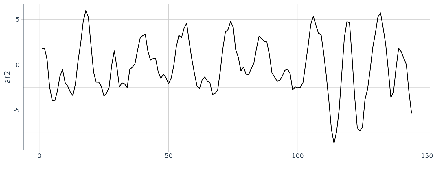
[1]  12 -12

To simulate AR(2) with complex roots:

set.seed(8675309)
dat <- tsibble(
  t = 1:144,
  ar2 = arima.sim(
    list(order = c(2, 0, 0), ar = c(1.5, -.75)),      
    n = 144
  ),
  index = t
)

And plotting the ACF. Note that the ACF decreases exponentially and in a sinosoidal manner:

dat |>
  ACF(ar2) |>
  autoplot() +
  xlab("") +
  ylab("") +
  ggtitle("ACF") +     
  theme_tq()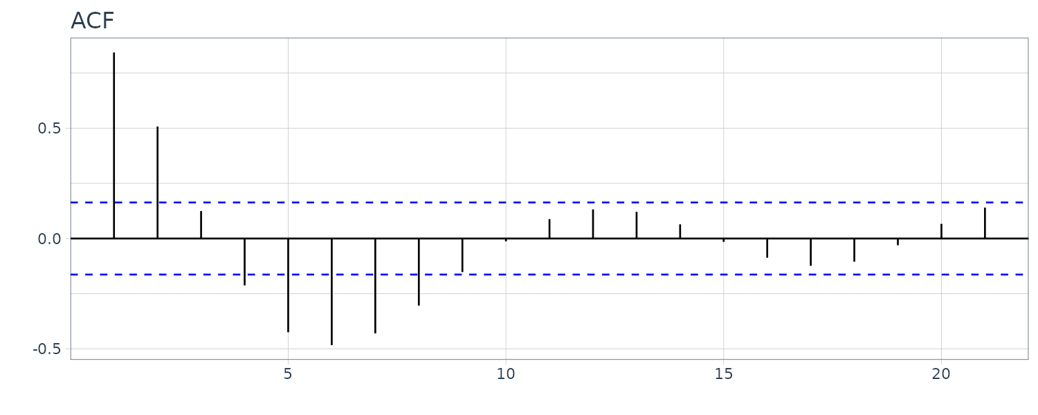

ARMA(p, q) \(\psi\)-weights

For a causal ARMA(p, q) model, where the zeros of \(\phi(z)\) are outside the unit circle:

\[\begin{aligned} \phi(B)x_{t} &= \theta(B)w_{t}\\ x_{t} &= \sum_{j = 0}^{\infty}\psi_{j}w_{t-j} \end{aligned}\]

To solve for the weights in general, we match the coefficients:

\[\begin{aligned} (1 - phi_{1}z - \phi_{2}z^{2} - \cdots -\phi_{p}z^{p})(\psi_{0} + \psi_{z} + \psi_{2}z^{2} + \cdots) &= (1 + \theta_{1}z + \theta_{2}z^{2} + \cdots) \end{aligned}\] \[\begin{aligned} \psi_{0} &= 1\\ \psi_{1} - \phi_{1}\psi_{0} &= \theta_{1}\\ \psi_{2} - \phi_{1}\psi_{1} - \phi_{2}\psi_{0} &= \theta_{2}\\ \psi_{3} - \phi_{1}\psi_{2} - \phi_{2}\psi_{1} - \phi_{3}\psi_{0} &= \theta_{3}\\ \cdots \end{aligned}\]

The \(\psi\)-weights satisfy the following homogeneous difference equation:

\[\begin{aligned} \psi_{j} - \sum_{k=1}^{p}\phi_{k}\psi_{j-k} &= 0\\ j &\geq \text{max}(p, q + 1) \end{aligned}\]

With initial conditions:

\[\begin{aligned} \psi_{j} - \sum_{k=1}^{p}\phi_{k}\psi_{j-k} &= \theta_{j} \end{aligned}\]

Consider the ARMA process:

\[\begin{aligned} x_{t} &= 0.9x_{t-1} + 0.5w_{t-1} + w_{t}\\ \end{aligned}\]

With:

\[\begin{aligned} \text{max}(p, q + 1) &= 2 \psi_{0} - 0 &= 1\\ \psi_{1} - \phi_{1}\psi_{0} &= 0.5\\ \psi_{1} &= 0.5 + 0.9 \times 1\\ &= 1.4 \end{aligned}\]

The remaining \(\psi\)-weights:

\[\begin{aligned} \psi_{j} - 0.9\psi_{j-1} &= 0\\ \psi_{2} &= 0.9 \times 1.4\\ \psi_{3} &= 1.4(0.9^{2})\\ \vdots\\ \psi_{j} &= 1.4(0.9^{j-1})\\ \end{aligned}\]

ACF of ARMA(p, q) Process

For a causal ARMA(p, q) model:

\[\begin{aligned} x_{t} &= \sum_{j=0}^{\infty}\psi_{j}w_{t-j} \end{aligned}\]

It follows that:

\[\begin{aligned} E[x_{t}] &= 0\\ \gamma(h) &= \text{cov}(x_{t+h}, x_{t})\\ &= \sigma_{w}^{2}\sum_{j=0}^{\infty}\psi_{j}\psi_{j+h} \end{aligned}\]

We can solve the \(\psi\)-weights like how we did above previously.

It is also possible to obtain a homogeneous difference equatoion directly in terms of \(\gamma(h)\).

First note that:

\[\begin{aligned} \text{cov}(w_{t+h-j}, x_{t}) &= \ext{cov}\Big(\psi_{k}w_{t-k}\Big)\\ &= \psi_{j-h}\sigma_{w}^{2} \end{aligned}\]

Then:

\[\begin{aligned} \gamma(h) &= \text{cov}(x_{t+h}, x_{t})\\ &= \text{cov}\Big(\sum_{j=1}^{p}\phi_{j}x_{t+h-j} + \sum_{j=0}^{q}\theta_{j}w_{t+h-j}, x_{t}\Big)\\ &= \sum_{j=1}^{p}\phi_{j}\gamma(h-j) + \sigma_{w}^{2}\sum_{j=h}^{q}\theta_{j}\psi_{j-h}\\ h &\geq 0 \end{aligned}\]

Thus for \(h \geq \text{max}(p, q + 1)\):

\[\begin{aligned} \gamma(h) - \phi_{1}\gamma(h-1) - \cdots - \phi_{p}\gamma(h-p) &= 0\\ \end{aligned}\]

And for \(0 \leq h < \textrm{max}(p, q+1)\) initial conditions:

\[\begin{aligned} \gamma(h) - \sum_{j=1}^{p}\phi_{j}\gamma(h-j) &= \sigma_{w}^{2}\sum_{j=h}^{q}\theta_{j}\psi_{j-h} \end{aligned}\]

ACF of AR(p)

For the general case:

\[\begin{aligned} x_{t} = \phi_{1}x_{t-1} + \cdots + \phi_{p}x_{t-p} + w_{t} \end{aligned}\]

It follows that:

\[\begin{aligned} \rho(h) - \phi_{1}\rho(h - 1) - \cdots - \phi(p)\rho(h-p) &= 0\\ h &\geq p \end{aligned}\]

The general solution to the above difference solution (\(z_{j}\) are roots of \(\phi(x)\)):

\[\begin{aligned} \rho(h) &= z_{1}^{-h}P_{1}(h) + \cdots + z_{r}^{-h}P_{r}(h)\\ m_{1} + \cdots + m_{r} &= p\\ \end{aligned}\]

Where \(P_{j}(h)\) is a polynomial in h\(of degree\)m_{j}-1$$.

ACF of ARMA(1, 1)

Consider the ARMA(1, 1) process:

\[\begin{aligned} x_{t} &= \phi x_{t-1} + \theta w_{t-1} + w_{t}\\ |\phi| &< 1 \end{aligned}\]

It follows from the difference model solution:

\[\begin{aligned} \gamma(h) &= c\phi^{h} \end{aligned}\]

The initial conditions, we use the equations for the generic ARMA(p, q):

\[\begin{aligned} \gamma(0) &= \phi \gamma(1) + \sigma_{w}^{2}[1 + \theta \phi + \theta^{2}]\\ \gamma(1) &= \phi \gamma(0) + \sigma_{w}^{2}\theta \end{aligned}\]

Solving for \(\gamma(0)\) and \(\gamma(1)\):

\[\begin{aligned} \gamma(0) &= \sigma_{w}^{2}\frac{1 + 2\theta\phi + \theta^{2}}{1 - \phi^{2}}\\ \gamma(1) &= \sigma_{w}^{2}\frac{(1 + \theta \phi)(\phi + \theta)}{1 - \phi^{2}} \end{aligned}\]

The specific solution for \(h \geq 1\):

\[\begin{aligned} \gamma(1) &= c\phi\\ c &= \frac{\gamma(1)}{\phi}\\ \gamma(h) &= \frac{\gamma(1)}{\phi}phi^{h}\\ &= \sigma_[w]^{2}\frac{(1 + \theta \phi)(\phi + \theta)}{1 - \phi^{2}}\phi^{h-1} \end{aligned}\]

Dividing by \(\gamma(0)\):

\[\begin{aligned} \rho(h) &= \frac{\gamma(h)}{\gamma(0)}\\ &= \frac{\sigma_[w]^{2}\frac{(1 + \theta \phi)(\phi + \theta)}{1 - \phi^{2}}\phi^{h-1}}{\sigma_{w}^{2}\frac{1 + 2\theta\phi + \theta^{2}}{1 - \phi^{2}}}\\ &= \frac{(1 + \theta \phi)(\phi + \theta)}{1 + 2\theta\phi + \theta^{2}}\phi^{h-1} \end{aligned}\]

Note that the ACF for ARMA(1, 1) is the same as AR(1).

Partial Autocorrelation Function (PACF)

Recall that if \(X, Y, Z\) are random variables, the the partial correlation between \(X, Y\) given \(Z\) is obtained by regressing \(X\) on \(Z\) to obtain \(\hat{X}\), and similarly \(\hat{Y}\) and calculating the partial correlation:

\[\begin{aligned} \rho_{XY|Z} &= \text{corr}(X - \hat{X}, Y - \hat{Y}) \end{aligned}\]

If the variables are also multivariate normal, then:

\[\begin{aligned} \rho_{XY|Z} &= \text{corr}(X, Y|Z) \end{aligned}\]

For a causal AR(1) model, we can see that:

\[\begin{aligned} x_{t} &= \phi x_{t-1} + w_{t}\\ \gamma_{x}(2) &= \text{cov}(x_{t}, x_{t-2})\\ &= \text{cov}(\phi x_{t-1} + w_{t}, x_{t-2})\\ &= \text{cov}(\phi^{2} x_{t-2} + \phi w_{t-1} + w_{t}, x_{t-2})\\ &= \phi^{2}\gamma_{x}(0) \end{aligned}\]

Note that because of causality, \(x_{t-2}\) is uncorrelated with \(w_{t}, w_{t-1}\). We can see that the autocovariance between \(x_{t}, x_{t-2}\) is not zero.

But what if we consider the autocovariance between \(x_{t} - \phi x_{t-1}\) and \(x_{t-2} - \phi x_{t-1}\)? That is the covariance between \(x_{t}, x_{t-2}\) with the linear dependence of each on \(x_{t-1}\) removed:

\[\begin{aligned} \text{cov}(x_{t} - \phi x_{t-1}, x_{t-2} - \phi x_{t-1})\\ &= \text{cov}(w_{t}, x_{t-1} - \phi x_{t-1})\\ &= 0 \end{aligned}\]

Let \(\hat{x_{t+h}}\) denote the regression of \(x_{t+h}\) on \(\{x_{t+h-1}, \cdots, x_{t+1}\}\):

\[\begin{aligned} \hat{x}_{t+h} &= \beta_{1}x_{t+h-1} + \beta_{2}x_{t+h-2} + \cdots + \beta_{h-1}x_{t+1} \end{aligned}\]

Because of stationarity, we can show that:

\[\begin{aligned} \hat{x}_{t} &= \beta_{1}x_{t+1} + \beta_{2}x_{t+2} + \cdots + \beta_{h-1}x_{t+h-1} \end{aligned}\]

The PACF of a stationary process \(x_{t}\) is denoted as \(\phi_{hh}\):

\[\begin{aligned} \phi_{hh} &= \text{corr}(x_{t+h} - \hat{x_{t+h}}, x_{t} - \hat{x_{t}})\\ h &\geq 2\\ \phi_{11} &= \text{corr}(x_{t+1}, x_{t}) \end{aligned}\]

If the process is further Gaussian, then:

\[\begin{aligned} \phi_{hh} &= \text{corr}(x_{t+h}, x_{t}|x_{t+1}, \cdots, x_{t+h-1}) \end{aligned}\]

Example: The PACF of AR(1)

Consider:

\[\begin{aligned} x_{t} &= \phi x_{t-1} + w_{t}\\ |\phi| &<1 \end{aligned}\]

By definition:

\[\begin{aligned} \phi_{11}&= \rho(1) \\ &= \phi \end{aligned}\]

We choose \(\beta\) to minimize:

\[\begin{aligned} E[(x_{t+2} - \hat{x}_{t+2})^{2}] &= E[(x_{t+2} - \beta x_{t+1})^{2}]\\ &= E[x_{t+2}^{2}] - 2\beta E[x_{t+2}x_{t+1}] + \beta^{2}E[x_{t+1}^{2}]]\\ &= \gamma(0) - 2\beta \gamma(1) + \beta^{2}\gamma(0) \end{aligned}\]

PACF of AR(p)

Consider the AR(p) model:

\[\begin{aligned} x_{t+h} &= \sum_{j=1}^{p}\phi_{j}x_{t+h-j} + w_{t+h} \end{aligned}\]

The regression of \(x_{t+h}\) on \(\{x_{t+1, \cdots, x_{t+h-1}}\}\) when \(h > p\) is:

\[\begin{aligned} \hat{x}_{t+h} &= \sum_{j=1}^{p}\phi_{j}x_{t+h-j} \end{aligned}\]

And when \(h > p\):

\[\begin{aligned} \phi_{hh} &= \text{corr}(x_{t+h} - \hat{x_{t+h}, x_{t-\hat{x}_{t}}})\\ &= \text{corr}(w_{t+h}, x_{t} - \hat{x}_{t}) &= 0 \end{aligned}\]

When \(h \leq p\), we will show later that:

\[\begin{aligned} \phi_{pp} &= \phi_{p} \end{aligned}\]

Let’s plot the ACF and PACF for \(\phi_{1} = 1.5\) and \(\phi_{2} &= -0.75\):

\[\begin{aligned} dat <- tibble( acf = ARMAacf(ar = c(1.5, -.75), ma = 0, 24)[-1], pacf = ARMAacf(ar = c(1.5, -.75), ma = 0, 24, pacf = TRUE), lag = 1:24 ) \end{aligned}\]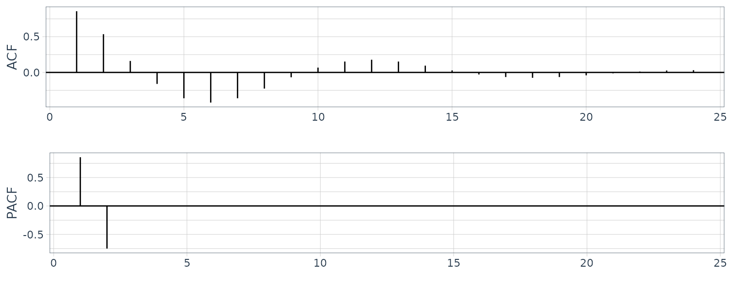

For an invertible MA(q) model, we can write as an infinite AR model:

\[\begin{aligned} x_{t} &= -\sum_{j=1}^{\infty}\pi_{j}x_{t-j} + w_{t} \end{aligned}\]

We can show that for MA(1) model in general, the PACF:

\[\begin{aligned} \phi_{hh} &= -\frac{(-\theta)^{h}(1 - \theta^{2})}{1 - \theta^{2(h + 1)}}\\ h &\geq 1 \end{aligned}\]

The PACF for MA models behave like ACF for AR models. Also, the PACF for AR models behave like ACF for MA models.

Preliminary Analysis of the Recruitment Series

Let’s look at the ACF and PACF of the Recruitment series:

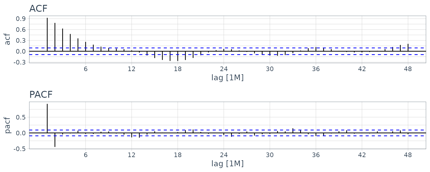
The ACF seem to have roughly 12-month period cycles. PACF only have 2 main signficant values. This suggest a AR(2) model:

\[\begin{aligned} x_{t} &= \phi_{0} + \phi_{1}x_{t-1} + \phi_{2}x_{t-2} + w_{t} \end{aligned}\]

Next we fit the model and get the following coefficients:

\[\begin{aligned} \hat{\phi}_{0} &= 6.80_{(0.44)}\\ \hat{\phi}_{1} &= 1.35_{(0.0416)}\\ \hat{\phi}_{2} &= -0.46_{(0.0417)}\\ \hat{\sigma}_{w}^{2} &= 89.9 \end{aligned}\]

fit <- rec |>
  model(
    ARIMA(value ~ pdq(2, 0, 0) + PDQ(0, 0, 0))
  )

> coef(fit)
# A tibble: 3 × 6
  .model                                     term     estimate std.error statistic   p.value
  <chr>                                      <chr>       <dbl>     <dbl>     <dbl>     <dbl>
1 ARIMA(value ~ pdq(2, 0, 0) + PDQ(0, 0, 0)) ar1         1.35     0.0416      32.5 1.98e-120
2 ARIMA(value ~ pdq(2, 0, 0) + PDQ(0, 0, 0)) ar2        -0.461    0.0417     -11.1 2.29e- 25
3 ARIMA(value ~ pdq(2, 0, 0) + PDQ(0, 0, 0)) constant    6.80     0.440       15.4 1.48e- 43     

> fit |>
  glance() |>
  pull(sigma2)
    year 
89.92993 

Forecasting

In forecasting, the goal is to predict future values of a time series \(x_{n+m}\), given data collected to the present:

\[\begin{aligned} x_{1:n} &= {x_{1}, x_{2}, \cdots, x_{n}} \end{aligned}\]

We will assume the time series is stationary. We define the minimum mean square error predictor as:

\[\begin{aligned} x_{n+m}^{n} &= E[x_{n+m}|x_{1:n}] \end{aligned}\]

It is the minimum because the conditional expectation minimizes the mean square error:

\[\begin{aligned} E[(x_{n+m} - g(x_{1:n})^{2}] \end{aligned}\]

Where \(g(x_{1:n})\) is a function of the observations.

The Best Linear Predictor (BLP):

\[\begin{aligned} x_{n+m}^{n} &= \alpha_{0} + \sum_{k=1}^{n}\alpha_{k}x_{k} \end{aligned}\]

Is found by solving:

\[\begin{aligned} E[(x_{n+m} - x_{n+m}^{n})x_{k}] &= 0 \end{aligned}\]

This can be shown by using least squares.

By taking expectation:

\[\begin{aligned} \mu &= \alpha_{0} + \sum_{k=1}^{n}\alpha_{k}\mu\\ \alpha_{0} &= \mu\Big(1 - \sum_{k=1}^{n}\alpha_{k}\Big) \end{aligned}\]

Hence, the BLP is:

\[\begin{aligned} x_{n+m}^{n} &= \mu + \sum_{k=1}^{n}\alpha_{k}(x_{k} - \mu) \end{aligned}\]

There is no loss of generality in considering the case that \(\mu = 0\) which result in \(\alpha_{0} = 0\).

We first consider the one-step-ahead prediction. We wish to forecast \(x_{n+1}\) given \(\{x_{1}, \cdots, x_{n}\}\). Taking \(m=1\) and taking \(\mu = 0\):

\[\begin{aligned} x_{n+1}^{n} &= \sum_{k=1}^{n}\alpha_{k}(x_{k} - \mu)\\ \alpha_{k} &= \phi_{n, n+1-k} \end{aligned}\]

We would want the coefficients to satisfy:

\[\begin{aligned} x_{n+1}^{n} &= \phi_{n1}x_{n} + \phi_{n2}x_{n-1} + \cdots + \phi_{nn}x_{1} \end{aligned}\] \[\begin{aligned} E\Big[\Big(x_{n+1} - \sum_{j=1}^{n}\phi_{nj}x_{n+1-j}\Big)x_{n+1-k}\Big] &= 0\\ E[x_{n+1}x_{n+1-k}] - E\Big[\sum_{j=1}^{n}\phi_{nj}x_{n+1-j} x_{n+1-k}\Big] & = 0\\ \sum_{j= 1}^{n}\phi_{nj}\gamma(k - j) - \gamma(k) &= 0\\ \sum_{j= 1}^{n}\phi_{nj}\gamma(k - j) &= \gamma(k) \end{aligned}\]

We can represent this in matrix form:

\[\begin{aligned} \Gamma_{n}\boldsymbol{\phi}_{n} &= \boldsymbol{\gamma}_{n}\\ \Gamma_{n} &= \{\gamma(k - j)\}_{j, k = 1}^{n}\\ \boldsymbol{\phi}_{n} &= \begin{bmatrix} \phi_{n1}\\ \vdots\\ \phi_{nn} \end{bmatrix}\\ \boldsymbol{\gamma}_{n} &= \begin{bmatrix} \gamma(1)\\ \vdots\\ \gamma(n) \end{bmatrix}\\ \end{aligned}\]

The matrix \(\Gamma_{n}\) is nonnegative definite. If the matrix is nonsingular, the elements of \(\phi_{n}\) are unique and:

\[\begin{aligned} \phi_{n} &= \Gamma^{-1}\gamma_{n}\\ x_{n+1}^{n} &= \phi_{n}'x \end{aligned}\]

The mean square one-step-ahead prediction error is:

\[\begin{aligned} P_{n+1}^{n} &= E[(x_{n+1} - x_{n+1}^{n})^{2}]\\ &= E[(x_{n+1} - \phi_{n}'x)^{2}]\\ &= E[(x_{n+1} - \gamma_{n}'\Gamma_{n}^{-1}x)^{2}]\\ &= E[x_{n+1}^{2} - 2\gamma_{n}'\Gamma_{n}^{-1}x x_{n+1} + \gamma_{n}'\Gamma_{n}^{-1}x x' \Gamma_{n}^{-1}\gamma_{n}]\\ &= \gamma(0) - 2\gamma_{n}'\Gamma_{n}^{-1}\gamma_{n} + \gamma_{n}'\Gamma_{n}^{-1}\Gamma_{n}^{-1}\gamma_{n}\\ &= \gamma(0) - \gamma_{n}'\Gamma_{n}^{-1}\gamma_{n} \end{aligned}\]

Example: Prediction of an AR(2) Model

Suppose we have a causal AR(2) process:

\[\begin{aligned} x_{t} &= \phi_{1}x_{t-1} + \phi_{2}x_{t-2} + w_{t} \end{aligned}\]

Then:

\[\begin{aligned} x_{2}^{1} &= \phi_{11}x_{1}\\ \sum_{j=1}^{n = }\phi_{11}\gamma(k - j) &= \gamma(k)\\ k &= 1\\ \phi_{11}\gamma(0) &= \gamma(1)\\ \phi_{11} &= \frac{\gamma(1)}{\gamma(0)}\\ &= \rho(1) \end{aligned}\]

Now if we want the prediction of \(x_{3}\):

\[\begin{aligned} \phi_{21}\gamma(0) + \phi_{22}\gamma(1) &= \gamma(1)\\ \phi_{21}\gamma(1) + \phi_{22}\gamma(0) &= \gamma(2)\\[5pt] \begin{bmatrix} \phi_{21}\\ \phi_{22} \end{bmatrix} &= \begin{bmatrix} \gamma(0) & \gamma(1)\\ \gamma(1) & \gamma(0) \end{bmatrix}^{-1} \begin{bmatrix} \gamma(1)\\ \gamma(2) \end{bmatrix}\\ \end{aligned}\]

We can easily show that:

\[\begin{aligned} \phi_{21} &= \phi_{1} \phi_{22} &= \phi_{2} \end{aligned}\]

As:

\[\begin{aligned} E\Big[\Big(x_{3} - (\phi_{x2} + \phi_{2}x_{1})\Big)x_{1}\Big]\\ &= E[w_{3}]x_{1}\\ &= 0\\ E\Big[\Big(x_{3} - (\phi_{x2} + \phi_{2}x_{1})\Big)x_{2}\Big]\\ &= E[w_{3}]x_{2}\\ &= 0 \end{aligned}\]

The noise is independent from the explanatory variables.

This could be generalize for \(n \geq 2\):

\[\begin{aligned} x_{n+1}^{n} &= \phi_{1}x_{n} + \phi_{2}x_{n-1} \end{aligned}\]

And further generalize to AR(p) model:

\[\begin{aligned} x_{n+1}^{n} &= \phi_{1}x_{n} + \phi_{2}x_{n-1} + \cdots + \phi_{p}x_{n-p+1} \end{aligned}\]

For ARMA models, the prediction euqations will not be as simple as the pure AR case.

The Durbin-Levinson Algorithm

For large n, the inversion of a large matrix is prohibitive. However we can use iterative solutions such as Durbin-Levison algorithm. \(\phi_{n}\) and the mean square one-step-ahead prediction error \(P_{n+1}^{n}\) can be solved iteratlively as follows:

\[\begin{aligned} \phi_{00} &= 0\\ P_{1}^{0} &= \gamma(0) \end{aligned}\]

For \(n \geq 1\):

\[\begin{aligned} \phi_{nn} &= \frac{\rho(n) - \sum_{k = 1}^{n-1}\phi_{n-1, k}\rho(n-k)}{1 - \sum_{k=1}^{n-1}\phi_{n-1,k}\rho(k)}\\ P_{n+1}^{n} &= P_{n}^{n-1}(1 - \phi_{nn}^{2}) \end{aligned}\]

For \(n \geq 2\):

\[\begin{aligned} \phi_{nk} &= \phi_{n-1, k} - \phi_{nn}\phi_{n-1, n-k} \end{aligned}\]

To start:

\[\begin{aligned} \phi_{00} &= \rho(1)\\ P_{2}^{0} &= \gamma(0) \end{aligned}\]

For \(n = 1\):

\[\begin{aligned} \phi_{11} &= \rho(1)\\ P_{2}^{1} &= \gamma(0)(1 - \phi_{11}^{2}) \end{aligned}\]

For \(n = 2\):

\[\begin{aligned} \phi_{22} &= \frac{\rho(2) - \phi_{11}\rho(1)}{1 - \phi_{11}\rho(1)}\\ \phi_{21} &= \phi_{11}- \phi_{22}\phi_{11}\\ P_{3}^{2} &= P_{2}^{1}(1 - \phi_{22}^{2})\\ &= \gamma(0)(1 - \phi_{11}^{2})(1 - \phi_{22}^{2}) \end{aligned}\]

For \(n = 3\):

\[\begin{aligned} \phi_{33} &= \frac{\rho(3) - \phi_{21}\rho(2) - \phi_{22}\rho(1)}{1 - \phi_{21}\rho(1) - \phi_{22}\rho(2)}\\ \phi_{32} &= \phi_{22}- \phi_{33}\phi_{21}\\ \phi_{31} &= \phi_{21} - \phi_{33}\phi_{22}\\ P_{4}^{3} &= P_{3}^{2}(1 - \phi_{33}^{2})\\ &= \gamma(0)(1 - \phi_{11}^{2})(1 - \phi_{22}^{2})(1 - \phi_{33}^{2}) \end{aligned}\]

In general, the standard error is:

\[\begin{aligned} P_{n+1}^{n} &= \gamma(0)\Prod_{j=1}^{n}(1 - \phi_{jj}^{2}) \end{aligned}\]

The PACF of a stationary process \(x_{t}\) can be obtained iteratively from the coefficient \(\phi_{nn}\). For an AR(p) model:

\[\begin{aligned} x_{p+1}^{p} &= \phi_{p1}x_{p} + \phi_{p2}x_{p-1} + \cdots + \phi_{pp}x_{1}\\ &= \phi_{1}x_{p} + \phi_{2}x_{p-1} + \cdots + \phi_{p}x_{1} \end{aligned}\]

The PACF can just be lifted off the coefficients.

To show this for AR(2), recall that:

\[\begin{aligned} \rho(h) - \phi_{1}\rho(h - 1) - \phi_{2}rho(h-2) &= 0\\ \rho(1) &= \frac{\phi_{1}}{1 - \phi_{2}}\\ \rho(2) &= \phi_{1}\rho(1) + \phi_{2} \end{aligned}\] \[\begin{aligned} \rho(3) - \phi_{1} - \phi_{2}\rho(1) &= 0 \end{aligned}\] \[\begin{aligned} \phi_{11} &= \rho(1) &= \frac{\phi_{1}}{1 - \phi_{2}}\\ \phi_{22} &= \frac{\rho(2) - \rho(1)^{2}}{1 - \rho(1)^{2}}\\ &= \frac{\Big(\phi_{1}\frac{\phi_{1}}{1 - \phi_{2}} + \phi_{2}\Big) - \Big(\frac{\phi_{1}}{1 - \phi_{2}}\Big)^{2}}{1 - \Big(\frac{\phi_{1}}{1 - \phi_{2}}\Big)^{2}}\\ &= \phi_{2}\\ \phi_{21} &= \rho(1)(1 - \phi_{2}) &= \phi_{1}\\ \phi_{33} &= \frac{\rho(3) - \phi_{1} - \phi_{2}\rho(1)}{1 - \phi_{1}\rho(1) - \phi_{2}\rho(2)}\\ &= 0 \end{aligned}\]

For a m-step-ahead predictor:

\[\begin{aligned} x_{n+m}^{n} &= \phi_{n1}^{(m)}x_{n} + \phi_{n2}^{(m)}x_{n - 1} + \cdots + \phi_{nn}^{(m)}x_{1} \end{aligned}\]

Satisfying the prediction equations:

\[\begin{aligned} E\Big[\Big(x_{n+m} - \sum_{j=1}^{n}\phi_{nj}^{(m)}x_{n+1-j}\Big)x_{n+1-k}\Big] &= 0\\ E[x_{n+m}x_{n+1-k}] - \sum_{j=1}^{n}\phi_{nj}^{(m)}E[x_{n+1-j}x_{n+1 - k}] &= 0 \end{aligned}\] \[\begin{aligned} \sum_{j=1}^{n}\phi_{nj}^{(m)}E[x_{n+1-j}x_{n+1-k}] &= E[x_{n+m}x_{n+1-k}]\\ \sum_{j=1}^{n}\phi_{nj}^{(m)}\gamma(k - j) &= \gamma(m + k -1) k &= 1, \cdots, n \end{aligned}\]

The prediction equations can be written in matrix notation:

\[\begin{aligned} \Gamma_{n}\boldsymbol{\phi}_{n}^{(m)} &= \boldsymbol{\gamma}_{n}^{(m)} \end{aligned}\]

The mean square m-step-ahead prediction error is:

\[\begin{aligned} P_{n+m}^{n} &= E[(x_{n+m} - x_{n+m}^{n})^{2}]\\ &= \gamma(0) - \boldsymbol{\gamma}_{n}(m)'\Gamma_{n}^{-1}\boldsymbol{\gamma}_{n}^{(m)} \end{aligned}\]

Innovations Algorithm

The innovations:

\[\begin{aligned} x_{t} - x_{t}^{t-1}\\ x_{s} - x_{s}^{s-1}\\ \end{aligned}\]

They are uncorrelated for \(s\neq t\)

The one-step-ahead predictors and their mean-squared errors can be calculated iteratively as:

\[\begin{aligned} x_{1}^{0} &= 0\\ x_{t+1}^{t} &= \sum_{j=1}^{t}\theta_{tj}(x_{t+1} - j - x_{t+1-j}^{t-j})\\ P_{1}^{0} &= \gamma(0)\\ P_{t+1}^{t} &= \gamma(0) - \sum_{j=0}^{t-1}\theta_{t,t-j}^{t-1}\theta_{t, t-j}^{2}P_{j+1}^{j}\\ \theta_{t, t-j} &= \frac{\gamma(t-j)-\sum_{k=0}^{j-1}\theta_{j, j-k}\theta_{t,t-k}P_{k+1}}{P_{j+1}^{j}} \end{aligned}\]

In the general case:

\[\begin{aligned} x_{n+m}^{n}&= \sum_{j=m}^{n+m-1}\theta_{n+m-1, j}(x_{n+m-j}- x_{n+m-j}^{n_m-j-1})\\ P_{n+m}^{n} &= \gamma(0) - \sum_{j = m}^{n+m-1}\theta_{n+m-1, j}^{2}P_{n+m-j}^{n+m-j-1}\\ \theta_{t, t-j} &= \frac{\gamma(t-j)-\sum_{k=0}^{j-1}\theta_{j, j-k}\theta_{t,t-k}P_{k+1}}{P_{j+1}^{j}} \end{aligned}\]

Consider an MA(1) model:

\[\begin{aligned} x_{t} &= w_{t} + \theta w_{t-1} \end{aligned}\]

We can show that:

\[\begin{aligned} \gamma(0) &= (1 + \theta^{2})\sigma_{w}^{2}\\ \gamma(1) &= \theta\sigma_{w}^{2}\\ \gamma(h) &= 0\\ \theta_{nj} &= 0\\ j &= 2, \cdots, n\\ \theta_{n1} &= \frac{\gamma(1) - 0}{P_{n}^{n-1}}\\ \frac{\theta\sigma_{w}^{2}}{P_{n}^{n-1}}\\ P_{1} &= (1 + \theta^{2})\sigma_{w}^{2}\\ P_{n+1}^{n} &= (1 + \theta^{2} - \theta\theta_{n1})\sigma_{w}^{2} \end{aligned}\]

Finally, the one-step-ahead predictor is:

\[\begin{aligned} x_{n+1}^{n} &= \frac{\theta(x_{n}-x_{n}^{n-1})\sigma_{w}^{2}}{P_{n}^{n-1}} \end{aligned}\]

Forecasting ARMA Processes

For ARMA models, it is easier to calculate the predictor of \(x_{n+m}\), assuming we have the complete history (infinite past):

\[\begin{aligned} \tilde{x}_{n+m}^{n} &= E[x_{n+m}|x_{n}, x_{n-1}, \cdots, x_{1}, x_{0}, x_{-1}, \cdots] \end{aligned}\]

For large samples, \(\tilde{x}_{n+m}\) is a good approximation to \(x_{n+m}^{n}\).

We can write \(x_{n+m}\) in its causal and invertible forms:

\[\begin{aligned} x_{n+m} &= \sum_{j=0}^{\infty}\psi_{j}w_{n+m-j}\\ \psi_{0} &= 1\\ w_{n+m} &= \sum_{j=0}^{\infty}\pi_{j}x_{n+m-j}\\ \pi_{0} &= 1 \end{aligned}\] \[\begin{aligned} \tilde{x}_{n+m}^{n} &= E[x_{n+m}|x_{n}, x_{n-1}, \cdots, x_{1}, x_{0}, x_{-1}, \cdots]\\ &= \sum_{j=0}^{\infty}\psi_{j}\tilde{w}_{n+m-j}\\ &= \sum_{j=m}&{\infty}\psi_{j}\tilde{w}_{n+m-j}\\ \end{aligned}\]

This is because:

\[\begin{aligned} \tilde{w}_{t} &= E[w_{t}|x_{n}, x_{n-1}, \cdots, x_{0}, x_{-1}, \cdots]\\ &= \begin{cases} 0 & t > n\\ w_{t} & t \leq n \end{cases} \end{aligned}\]

Similarly:

\[\begin{aligned} \tilde{w}_{n+m} &= \sum_{j=0}^{\infty}\pi_{j}\tilde{x}_{n+m-j}\\ &= \tilde{x}_{n+m} + \sum_{j=1}^{\infty}\pi_{j}\tilde{x}_{n+m-j}\\ &= 0\\ \tilde{x}_{n+m} &= -\sum_{j=1}^{\infty}\pi_{j}\tilde{x}_{n+m-j}\\ &= -\sum_{j=1}^{m-1}\pi_{j}\tilde{x}_{n+m-j} - \sum_{j=m}^{\infty}\pi x_{n+m-j} \end{aligned}\]

Because:

\[\begin{aligned} \tilde{x}_{t} &= E[x_{t}|x_{n}, x_{n-1}, \cdots, x_{0}, x_{-1}, \cdots] \\ &= x_{t}\\ t &\leq n \end{aligned}\]

Prediction is accomplished recursively, starting from \(M = 1\), and then continuing for \(m = 2, 3, \cdots\):

\[\begin{aligned} \tilde{x}_{n+m} &= -\sum_{j=1}^{\infty}\pi_{j}\tilde{x}_{n+m-j}\\ &= -\sum_{j=1}^{m-1}\pi_{j}\tilde{x}_{n+m-j} - \sum_{j=m}^{\infty}\pi x_{n+m-j} \end{aligned}\]

For the error:

\[\begin{aligned} x_{n+m} - \tilde{x}_{n+m} &= \sum_{j=0}^{\infty}\phi_{j}w_{n+m-j} - \sum_{j=m}^{\infty}\phi_{j}w_{n+m-j}\\ &= \sum_{j=0}^{m-1}\pi_{j}\phi_{j}w_{n+m-j} \end{aligned}\]

Hence, the mean-square prediction error is:

\[\begin{aligned} P_{n+m}^{n} &= E[x_{n+m} - \tilde{x}_{n+m}^{2}]\\ &= \sigma_{w}^{2}\sum_{j=0}^{m-1}\phi_{j}^{2} \end{aligned}\]

For a fixed sample size \(N\), the prediction errors are correlated:

\[\begin{aligned} E[(x_{n+m} - \tilde{x_{n+m}})(x_{n+m+k} - \tilde{x}_{n+m+k})] &= \sigma_{w}^{2}\sum_{j=0}^{m-1}\phi_{j}\phi_{j+k}\\ k & \geq 1 \end{aligned}\]

Consider forecasting an ARMA process with mean \(\mu_{x}\)

\[\begin{aligned} x_{n+m} - \mu_{x} &= \sum_{j=0}^{\infty}\psi_{j}w_{n+m-j}\\ x_{n+m} &= \mu_{x} + \sum_{j=0}^{\infty}\psi_{j}w_{n+m-j}\\ \tilde{x}_{n+m} &= \mu_{x} + \sum_{j=m}^{\infty}\psi_{j}w_{n+m-j}\\ \end{aligned}\]

As the \(\psi\)-weights dampen to 0 exponentially fast:

\[\begin{aligned} \lim_{m \rightarrow \infty}\tilde{x}_{n+m} \rightarrow \mu_{x} \lim_{m \rightarrow \infty}P_{n+m}^{n} &= \lim_{m \rightarrow \infty}\sigma_{w}^{2}\sum_{j=0}^{\infty}\psi_{j}^{2}\\ &= \gamma_{x}(0)\\ &= \sigma_{x}^{2} \end{aligned}\]

When \(n\) is small, the general prediction equations can be used:

\[\begin{aligned} x_{n+m}^{n} &= \alpha_{0} + \sum_{k=1}^{n}\alpha_{k}x_{k} \end{aligned}\]

And when \(n\) is large, we would use the above but by truncating as we do not observe \(x_{0}, x_{-1}, \cdots\):

\[\begin{aligned} \tilde{x}_{n+m}^{n} &\cong -\sum_{j=1}^{m-1}\pi_{j}\tilde{x}_{n+m-j} - \sum_{j=m}^{n+m-1}\pi x_{n+m-j} \end{aligned}\]

Truncated Prediction for ARMA

For ARMA(p, q) models, the truncated predictors for \(m = 1, 2, \cdots\):

\[\begin{aligned} \tilde{x}_{n+m}^{n} &= \phi_{1}\tilde{x}_{n+m - 1}^{n} + \cdots + \phi_{p}\tilde{x}_{n+m - p}^{n} + \theta_{1}\tilde{w}_{n+m-1}^{n} + \cdots + \theta_{q}\tilde{w}_{n+m-q}^{n}\\ 1 &\leq t \leq n\\ \tilde{x}_{t}^{n} &= 0\\ t \leq 0 \end{aligned}\]

The truncated prediction errors are given by:

\[\begin{aligned} \tilde{w}_{t}^{n} &= 0\\ t &\leq 0\\ t > n\\ \tilde{w}_{t}^{n} &= \phi(B)\tilde{x}_{t}^{n} - \theta_{1}\tilde{w}_{t-1}_^{n} - \cdots - \theta_{q}\tilde{w}_{t-q}_^{n}\\ 1 &\leq t \leq n \end{aligned}\]

Example: Forecasting an ARMA(1, 1) Series

Suppose we have the model:

\[\begin{aligned} x_{n+1} &= \phi x_{n} + w_{n+1} + \theta w_{n} \end{aligned}\]

The one-step-ahead truncated forecast is:

\[\begin{aligned} \tilde{x}_{n+1}^{n} &= \phi x_{n} + 0 + \theta \tilde{w}_{n}^{n} \end{aligned}\]

For \(m \geq 2\):

\[\begin{aligned} \tilde{x}_{n+m}^{n} &= \phi \tilde{x}_{n+m-1}^{n} \end{aligned}\]

To calculate \(\tilde{w}_{n}^{n}\), the model can be writen as:

\[\begin{aligned} w_{t} &= x_{t} - \phi x_{t-1} - \theta w_{t-1} \end{aligned}\]

For turncated forecasting:

\[\begin{aligned} \tilde{w}_{0}^{n} &= 0\\ x_{0} &= 0\\ \tilde{w}_{t}^{n} &= x_{t} - \phi x_{t-1} - \theta \tilde{w}_{t-1}^{n}\\ t &= 1, \cdots, n \end{aligned}\]

The \(\psi\)-weights satisfy:

\[\begin{aligned} \psi_{j} &= (\phi + \theta)\phi^{j-1} P_{n+m}^{n} &= \sigma_{w}^{2}\sum_{j=0}^{m-1}\psi_{j}^{2}\\ &= \sigma_{w}^{2}\Big[1 + (\phi + \theta)^{2}\sum_{j=1}^{m-1}\phi^{2(j-1)}\Big]\\ &= \sigma_{w}^{2}\Big[1 + \frac{(\phi + \theta)^{2}(1 - \phi^{2(m-1)})}{1 - \phi^{2}}\Big] \end{aligned}\]

The prediction intervals are of the form:

\[\begin{aligned} x_{n+m}^{n} \pm c_{\frac{\alpha}{2}}\sqrt{P_{n+m}^{n}} \end{aligned}\]

Forecasting the Recruitment Series

Using the parameter estimates as the actual parameter values:

\[\begin{aligned} x_{n+m}^{n} &= 6.74 + 1.35 x_{n+m-1}^{n}- 0.46x_{n+m-2}^{n} \end{aligned}\]

We have the following recurrence for the \(\psi\)-weights:

\[\begin{aligned} \psi_{j} &= 1.35\psi_{j-1} - 0.46 \psi_{j-2}\\ j &\geq 2\\ \psi_{0} &= 1\\ \psi_{1} &= 1.35 \end{aligned}\]

For \(n = 453\) and \(\hat{\sigma}_{w}^{2} = 89.72\):

\[\begin{aligned} P_{n+1}^{n} &= 89.72\\ P_{n+2}^{n} &= 89.72(\psi_{0} + \psi_{1})\\ &= 89.72(1 + 1.35^{2})\\ \psi_{2} &= 1.35 \times \psi_{1} - 0.46 \times \psi_{0}\\ &= 1.35^{2} - 0.46\\ P_{n+3}^{n} &= 89.72(\psi_{0} + \psi_{1} + \psi_{2})\\ &= 89.72(1 + 1.35^{2} + (1.35^{2} - 0.46)^{2}) \vdots \end{aligned}\]

fit <- rec |>
  model(ARIMA(value ~ pdq(2, 0, 0) + PDQ(0, 0, 0)))

> tidy(fit)
tidy(fit)
# A tibble: 3 × 6
  .model                                     term     estimate std.error statistic   p.value
  <chr>                                      <chr>       <dbl>     <dbl>     <dbl>     <dbl>
1 ARIMA(value ~ pdq(2, 0, 0) + PDQ(0, 0, 0)) ar1         1.35     0.0416      32.5 1.98e-120
2 ARIMA(value ~ pdq(2, 0, 0) + PDQ(0, 0, 0)) ar2        -0.461    0.0417     -11.1 2.29e- 25
3 ARIMA(value ~ pdq(2, 0, 0) + PDQ(0, 0, 0)) constant    6.80     0.440       15.4 1.48e- 43       

fit |>
  forecast(h = 24) |>
  autoplot(rec |> filter(year(index) > 1980)) +
  theme_tq()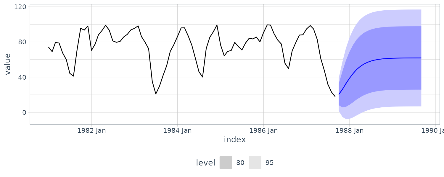

Backcasting

In backcasting, we are predicting past values:

\[\begin{aligned} x_{1-m}^{n} &= \sum_{j=1}^{n}\alpha_{j}x_{j} \end{aligned}\]

Analogous to the previous prediction equations, and assuming \(\mu_{x} = 0\):

\[\begin{aligned} \sum_{j=1}^{n}\alpha_{j}E[x_{j}x_{k}] &= E[x_{1-m}x_{k}]\\ \sum_{j=1}^{n}\alpha_{j}\gamma(k-j) &= \gamma(k - (m - 1)) k &= 1, \cdots, n \end{aligned}\]

And the backcasts are given by:

\[\begin{aligned} x_{1-m}^{n} &= \phi_{n1}^{(m)}x_{1} + \cdots + \phi_{nn}^{(m)}x_{n} \end{aligned}\]

As an example, we backcasted a simulated ARMA(1, 1) process:

\[\begin{aligned} set.seed(90210) dat <- tsibble( t = 1:100, x = arima.sim( list(order = c(1, 0, 1), ar = .9, ma = .5), n = 100 ), index = t ) backcasts <- dat |> mutate(reverse_time = rev(row_number())) |> update_tsibble(index = reverse_time) |> model(ARIMA(x ~ pdq(2, 0, 1) + PDQ(0, 0, 0))) |> forecast(h = 10) |> mutate(t = dat$t[1] - (1:10)) |> as_fable( index = t, response = "x", distribution = "x" ) backcasts |> autoplot(dat) + theme_tq() \end{aligned}\]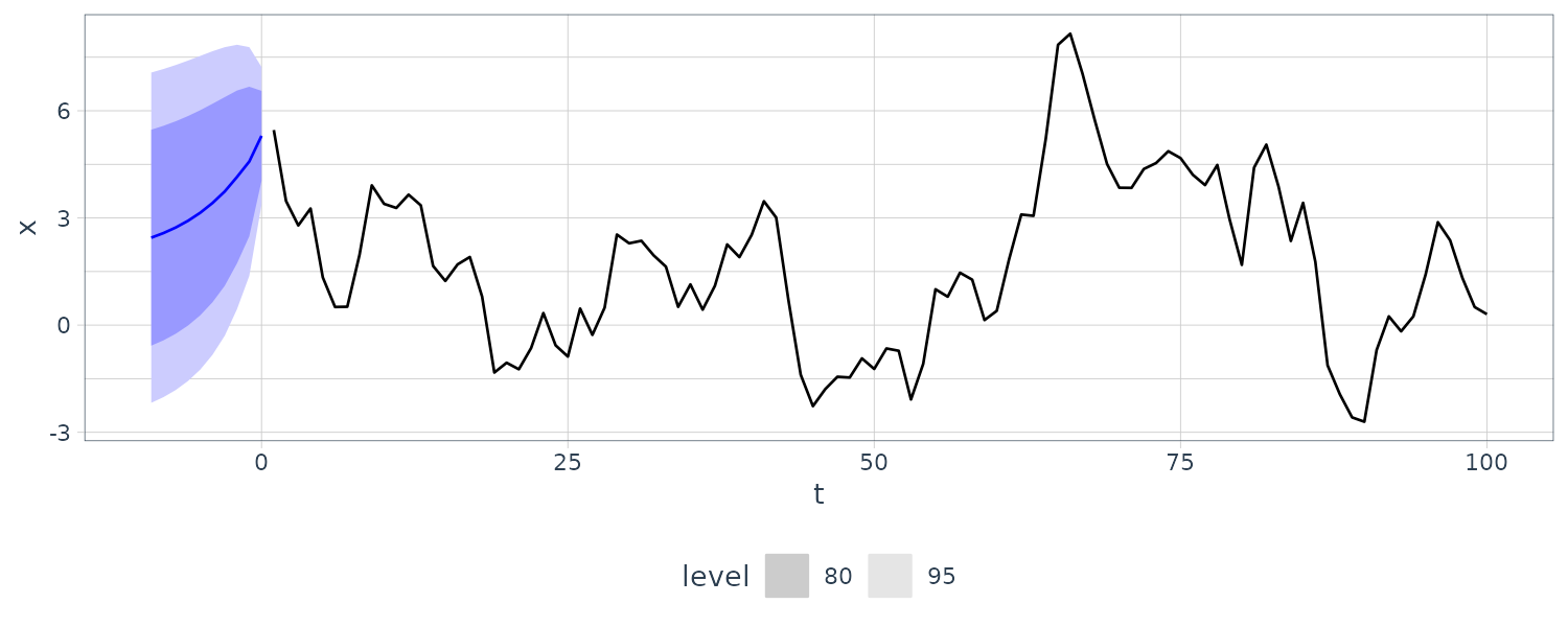

## Estimation

We would assume the ARMA(p, q) process is a causal and invertible Gaussian process and mean is 0. Our goal is to estimate the parameters:

\[\begin{aligned} \phi_{1}, \cdots, \phi_{p}\\ \theta_{1}, \cdots, \theta_{q}\\ \sigma_{w}^{2} \end{aligned}\]

Method of Moments Estimators

The idea is to equate population moments to sample moments and then solving for the parameters. THey can sometimes lead to suboptimal estimators.

We first consider the AR(p) models which the method of moments lead to optimal estimators.

\[\begin{aligned} x_{t} &= \phi_{1}x_{t-1} + \cdots + \phi_{p}x_{t-p} + w_{t} \end{aligned}\]

The Yule-Walker equations are:

\[\begin{aligned} \gamma(h) &= \phi_{1}\gamma(h-1) + \cdots + \phi_{p}\gamma(h-p)\\ h &= 1, 2, \cdots, p \end{aligned}\]

From the initial conditions:

\[\begin{aligned} \sigma_{w}^{2} &= \gamma(0) - \phi_{1}\gamma(1) - \cdots - \phi_{p}\gamma(p) \end{aligned}\]

And in matrix notation:

\[\begin{aligned} \Gamma_{p}\phi &= \boldsymbol{\gamma}_{p}\\ \sigma_{w}^{2} &= \gamma(0) - \bodsymbol{\phi}^{T}\boldsymbol{\gamma}_{p}\\ \Gamma_{p} &= \{\gamma(k-j)\}_{j, k =1}^{p}\\ \boldsymbol{\phi} &= (\phi_{1}, \cdots, \phi_{p})^{T}\\ \boldsymbol{\gamma}_{p} &= (\gamma(1), \cdots, \gamma(p))^{T} \end{aligned}\]

Yule-Walker estimators:

\[\begin{aligned} \hat{\boldsymbol{\phi}} &= \hat{\Gamma}_{p}^{-1}\hat{\boldsymbol{\gamma}_{p}}\\ \hat{\sigma}_{w}^{2} &= \hat{\gamma}(0) - \hat{\gamma}_{p}^{T}\hat{\Gamma}_{p}^{T}^{-1}\hat{\gamma}_{p} \end{aligned}\]

The Durbin-Levinson algorithm can be used to calculate \(\hat{\phi}\) without inverting.

Example: Yule–Walker Estimation for an AR(2) Process

Suppose we have the following AR(2) model:

\[\begin{aligned} x_{t} &= 1.5x_{t-1} - 0.75x_{t-2} + w_{t}\\ w_{t} &\sim \text{iid }N(0, 1)\\ \hat{\gamma}(0) &= 8.903\\ \hat{\rho}(1) &= 0.849\\ \hat{\rho}(2) &= 0.519 \end{aligned}\]

Thus:

\[\begin{aligned} \hat{\boldsymbol{\phi}} &= \begin{bmatrix} \hat{\phi}_{1}\\ \hat{\phi}_{2} \end{bmatrix}\\ &= \begin{bmatrix} 1 & 0.849\\ 0.849 & 1 \end{bmatrix}^{-1} \begin{bmatrix} 0.849\\ 0.519 \end{bmatrix}\\ &= \begin{bmatrix} 1.463\\ -0.723 \end{bmatrix}\\[5pt] \hat{\sigma}_{w}^{2} &= 8.903\Big[1 - (0.849, 0.519)\begin{bmatrix} 1.463\\ -0.723 \end{bmatrix}\Big]\\ &= 1.187 \end{aligned}\]

The asymptotic variance-covariance matrix of \(\hat{\boldsymbol{\phi}}\) is:

\[\begin{aligned} \frac{1}{144}\frac{1.187}{8.903}\begin{bmatrix} 0.058^{2} & -0.003\\ -0.003 & 0.058^{2} \end{bmatrix} \end{aligned}\]

Example: Yule–Walker Estimation of the Recruitment Series

We will fit an AR(2) model using Yule-Walker for the recruitment series in R:

\[\begin{aligned} rec <- as_tsibble(rec) rec <- as.ts(rec) rec.yw <- ar.yw(rec, order = 2) > rec.yw Call: ar.yw.default(x = rec, order.max = 2) Coefficients: 1 2 1.3316 -0.4445 Order selected 2 sigma^2 estimated as 94.8 > rec.yw$x.mean [1] 62.26278 > rec.yw$ar [1] 1.3315874 -0.4445447 > rec.yw$asy.var.coef [,1] [,2] [1,] 0.001783067 -0.001643638 [2,] -0.001643638 0.001783067 > rec.yw$var.pred [1] 94.79912 \end{aligned}\]

Plotting prediction:

\[\begin{aligned} rec <- as_tsibble(rec) dat <- as_tsibble(rec.pr$pred) |> rename(pred = value) |> mutate( lwr = pred - 1.96 * rec.pr$se, upr = pred + 1.96 * rec.pr$se ) rec |> autoplot() + geom_line( aes(x = index, y = pred), col = "blue", data = dat ) + geom_ribbon( aes(ymin = lwr, ymax = upr, y = pred), alpha = 0.1, fill = "blue", data = dat ) + theme_tq() \end{aligned}\]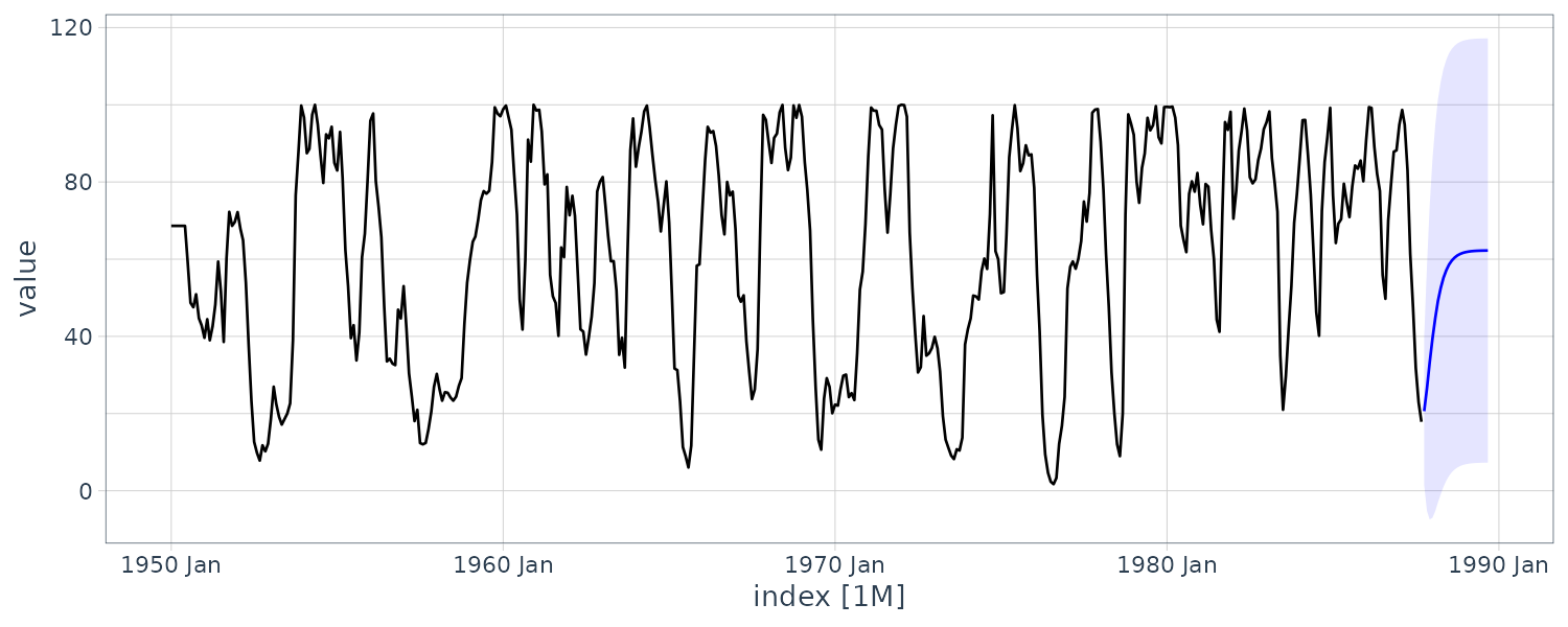

AR(p) models are linear models and the Yule-Walker estimators are essentially least squares estimators. If we use method of moments for MA or ARMA models, we will not get optimal estimators because such processes are nonlinear in the parameters.

Method of Moments Estimation for MA(1) Model

Consider the time series:

\[\begin{aligned} x_{t} &= w_{t} + \theta w_{t-1}\\ |\theta| &< 1 \end{aligned}\]

The model can then be rewritten as:

\[\begin{aligned} x_{t} &= \sum_{j=1}^{\infty}(-\theta)^{j}x_{t-j} + w_{t} \end{aligned}\]

Which is nonlinear in \(\theta\). The first two population autocovariances:

\[\begin{aligned} \gamma(0) &= \sigma_{w}^{2}(1 + \theta^{2})\\ \gamma(1) &= \sigma_{w}^{2}\theta \end{aligned}\]

Using the Durbin-Levinson algorithm:

\[\begin{aligned} \phi_{11} &= \rho(1)\\ \hat{\rho}(1) &= \frac{\hat{\gamma}(1)}{\hat{\gamma(0)}}\\ &= \frac{\hat{\theta}}{1 + \hat{\theta}^{2}} \end{aligned}\]

If \(\mid\hat{\rho}(1)\mid \leq \frac{1}{2}\), the solutions are real and otherwise a real solution does not exists. In the real solution case, the invertible estimate is:

\[\begin{aligned} \hat{\theta} &= \frac{1 - \sqrt{1 - 4\hat{\rho}}(1)^{2}}{2\hat{\rho}(1)} \end{aligned}\]

Maximum Likelihood and Least Squares Estimation

Let’s start with the causal AR(1) model:

\[\begin{aligned} x_{t} &= \mu + \phi(x_{t}- \mu)+ w_{t}\\ |\phi| &< 1\\ w_{t} &\sim \text{iid}N(0, \sigma_{w}^{2}) \end{aligned}\]

The likelihood:

\[\begin{aligned} L(\mu, \phi, \sigma_{w}^{2}) &= f(x_{1}, \cdots, x_{n}|\mu, \phi, \sigma_{w}^{2})\\ &= f(x_{1})f(x_{2}|x_{1})\cdots f(x_{n}|x_{n-1}) \end{aligned}\] \[\begin{aligned} x_{t}|x_{t-1} &\sim N(\mu + \phi(x_{t-1} - \mu), \sigma_{w}^{2})\\ f(x_{t}|x_{t-1}) &= f_{w}[(x_{t} - \mu)- \phi(x_{t-1} - \mu)]\\ L(\mu, \phi, \sigma_{w}) &= f(x_{1})\Prod_{t=2}^{n}f_{w}[(x_{t} - \mu)- \phi(x_{t-1} - \mu)]\\ \end{aligned}\]

We can show that:

\[\begin{aligned} L(\mu, \phi, \sigma_{w}^{2}) &= \frac{1}{(2\pi\sigma_{w}^{2})^{\frac{n}{2}}}(1 - \phi^{2})^{\frac{1}{2}}e^{-\frac{S(\mu, \phi)}{2\sigma_{w}^{2}}}\\ S(\mu, \phi) &= (1 - \phi^{2})(x_{1} - \mu)^{2} + \sum_{t=2}^{n}[(x_{t} - \mu) - \phi(x_{t-1}- \mu)]^{2} \end{aligned}\]

Taking the partial derivative of the log of the likelihood function with respect to \(\sigma_{w}^{2}\)$, we get:

\[\begin{aligned} l(\mu, \phi) &= \mathrm{log}\Big(\frac{S(\mu, \phi)}{n}) - \frac{\mathrm{log}(1 - \phi^{2})}{2}\\ &\propto -2 \mathrm{log}L(\mu, \phi, \hat{\sigma}_{w}{2}) \hat{\sigma}_{w}_^{2} &= \frac{S(\hat{\mu}, \hat{\phi})}{n} \end{aligned}\]

Where \(\hat{\mu}, \hat{\phi}\) are the MLEs.

In the case of AR models, we have the advantage that conditional on initial values, they are linear models:

\[\begin{aligned} L(\mu, \phi, \sigma_{w}^{2}|x_{1}) &= \Prod_{t=2}^{n}f_{w}[(x_{t} - \mu) - \phi(x_{t-1} - \mu)]\\ &= \frac{1}{2\pi \sigma_{w}^{2}}^{\frac{n-1}{2}e^{\frac{S_{c}(\mu, \phi)}{2\sigma_{w}^{2}}}} \end{aligned}\]

The MLE estimates are:

\[\begin{aligned} \hat{\mu} &= \frac{\bar{x}_{(2)} - \hat{\phi}\bar{x}_{(1)}}{1 - \hat{\phi}}\\ \hat{\phi}&= \frac{\sum_{t=2}^{n}(x_{t} - \bar{x}_{(2)})(x_{t-1} - \bar{x}_{(1)})}{\sum_{t=2}^{n}(x_{t-1} - \bar{x}_{(1)})^{2}}\\ \bar{x}_{(1)} &= \frac{\sum_{t=1}^{n-1}x_{t}}{n-1}\\ \bar{x}_{(2)} &= \frac{\sum_{t=2}^{n-1}x_{t}}{n-1}\\ \hat{\mu} &\cong \bar{x}\ \hat{\phi} &\cong \hat{\rho}(1) \end{aligned}\]

For general ARMA models, it is difficult to write the likelihood as an explicit function of the parameters, but easier to write in terms of the innovations \(x_{t} - x_{t}^{t-1}\).

Integrated Models for Nonstationary Data

If \(x_{t}\) is a random walk:

\[\begin{aligned} x_{t} &= x_{t-1} + w_{t}\\ \end{aligned}\]

We find that differencing \(x_{t}\) results in a stationary process:

\[\begin{aligned} \nabla x_{t} &= x_{t} - x_{t-1}\\ &= w_{t} \end{aligned}\]

We now consider a nonstationary trend component and a zero-mean stationary component:

\[\begin{aligned} x_{t} &= \mu_{t} + y_{t} \end{aligned}\]

Differencing such a process will lead to a stationary process:

\[\begin{aligned} \nabla x_{t} &= x_{t} - x_{t-1}\\ &= \beta_{0} + \beta_{1}t + y_{t} - \beta_{0} - \beta_{1}(t-1) - y_{t-1}\\ &= \beta_{1}(t - t + 1) + y_{t} - y_{t-1}\\ &= \beta_{1} + y_{t} - y_{t-1}\\ &= \beta_{1} + \nabla y_{t} \end{aligned}\]

Another model is the case in which \(\mu_{t}\) is stochastic and \(\nu_{t}\) is stationary:

\[\begin{aligned} \mu_{t} &= \mut_{t-1} + \nu_{t} \end{aligned}\]

In this case:

\[\begin{aligned} \nabla x_{t} &= \mu_{t} + y_{t}- \mu_{t-1} - y_{t-1}\\ &= \mu_{t-1} + \nu_{t} + \nabla y_{t} - \mu_{t-1}\\ &= \mu_{t} + \nabla y_{t} \end{aligned}\]

If instead of \(\mu_{t} = \beta_{0} + \beta_{1}t\), \(\mu_{t}\) is a k-th order polynomial:

\[\begin{aligned} \mu_{t} &= \sum_{j=0}^{k} \beta_{j}t^{j} \end{aligned}\]

Then \(\nabla^{k}x_{t}\) is stationary.

Stochastic trend modesls can lead to higher order differencing too. For example:

\[\begin{aligned} \mu_{t} &= \mu_{t-1} + \nu_{t}\\ \nu_{t} &= \nu_{t-1} + e_{t} \end{aligned}\]

Then:

\[\begin{aligned} \nabla^{2}x_{t} &= e_{t} + \nabla^{2}y_{t} \end{aligned}\]

Is stationary.

A process \(x_{t}\) is said to be ARIMA(p, d, q) if:

\[\begin{aligned} \nabla^{d}x_{t} &= (1 - B)^{d}x_{t} \end{aligned}\]

Is ARMA(p, q). In general, we write the model as:

\[\begin{aligned} \phi(B)(1 - B)^{d}x_{t}&= \theta(B)w_{t} \end{aligned}\]

But if \(E[\nabla^{d}x_{t}] = \mu\), then:

\[\begin{aligned} \phi(B)(1 - B)^{d}x_{t} &= \delta + \theta(B)w_{t}\\ \delta &= \mu(1 - \phi_{1} - \cdots - \phi_{p}) \end{aligned}\]

To obtain the forecasts, we write the ARMA process:

\[\begin{aligned} y_{t} &= \nabla^&{d}x_{t} \end{aligned}\]

For example, if \(d=1\):

\[\begin{aligned} y_{n+m}^{n} &= x_{n+m}^{n}- x_{n+m-1}^{n}\\ x_{n+m}^{n} &= y_{n+m}^{n} + x_{n+m=1}^{n} x_{n+1}^{n} &= y_{n+1}^{n} + x_{n} \end{aligned}\]

We can show that the mean-squared prediction error can be approximated by:

\[\begin{aligned} P_{n+m}^{n} &= \sigma_{w}^{2}\sum_{j=0}^{m-1}\phi_{j}^{*2}\\ \phi^{*}(z) &= \frac{\theta(z)}{\phi(z)}(1 - z)^{d} \end{aligned}\]

Example: Random Walk with Drift

Consider a random walk with drift (ARIMA(0, 1, 0)):

\[\begin{aligned} x_{t} &= \delta + x_{t-1} + w_{t}\\ x_{0} &= 0 \end{aligned}\]

The one-step-ahead forecast:

\[\begin{aligned} x_{n+1}^{n} &= E[x_{n+1}|x_{n}, \cdots, x_{1}]\\ &= E[\delta + x_{n} + w_{n+1}|x_{n}, \cdots, x_{1}]\\ &= \delta + x_{n} \end{aligned}\]

The two-step-ahead forecast:

\[\begin{aligned} x_{n+2}^{n} &= \delta + x_{n+1}^{n}\\ &= 2\delta + x_{n} \end{aligned}\]

In general, the m-step-ahead forecast:

\[\begin{aligned} x_{n+m}^{n} &= m\delta + x_{n} \end{aligned}\]

Recall that:

\[\begin{aligned} x_{n} &= n\delta + \sum_{j=1}^{n}w_{j}\\ x_{n+m} &= (n+m)\delta + \sum_{j=1}^{n+m}w_{j}\\ &= m\delta + x_{n} + \sum_{j=1}^{n+m}w_{j}\\ \end{aligned}\]

It follows that:

\[\begin{aligned} P_{n+m}^{n} &= E[x_{n+m} - x_{n+m}^{n}]^{2}\\ &= E[\sum_{j=1}^{n+m}w_{j}]^{2}\\ &= m\sigma_{w}^{2} \end{aligned}\]

As we can see the errors grow without bounds.

Example: ARIMA(0, 1, 1)

The ARIMA(0, 1, 1)model leads to the Exponentially Weighted Moving Averages, which is used in many economic time series:

\[\begin{aligned} x_{t} &= x_{t-1}+w_{t} - \lambda w_{t-1}\\ |\lambda| &< 1\\ x_{0} &= 0 \end{aligned}\]

Because \(\mid lambda\mid < 1\), \(y_{t}\) has an invertible representation:

\[\begin{aligned} y_{t} &= w_{t} - \lambda w_{t-1}\\ y_{t} &= \sum_{j=1}^{\infty}\lambda^{j}y_{t-j} + w_{t} \end{aligned}\]

For large \(t\) and putting \(x_{t} = 0\) for \(t\leq 0\), we can show that:

\[\begin{aligned} x_{t} &\cong \sum_{j=1}^{\inftye(1 - \lambda)\lambda^{j-1}}x_{t-j} + w_{t} \end{aligned}\]

Using the above approximation, we can calculate the approxiate one-step-ahead predictor

\[\begin{aligned} \tilde{x}_{n+1} &\cong \sum_{j=1}(1 - \lambda)\lambda^{j-1}x_{n+1-j}\\ &= (1 - \lambda)\lambda^{0}x_{n} + (1-\lambda)\lambda^{1}x_{n-1} + (1-\lambda)\lambda^{2}x_{n-2} + \cdots\\ &= (1 - \lambda)x_{n} + \lambda\sum_{j=1}^{\infty}(1 - \lambda)\lambda^{j-1}x_{n-j}\\ &= (1 - \lambda)x_{n}+ \lambda \tilde{x}_{n}\\ \end{aligned}\]

We can see the new forecast is a linear combination of the old forecast and the new observation. Since we only observe \(x_{1}, \cdots, x_{n}\):

\[\begin{aligned} \tilde{x}_{n+1}^{n} &= (1 - \lambda)x_{n}+ \lambda \tilde{x}_{n}^{n-1}\\ n & \geq 1\\ \tilde{x}_{1}^{0} &= x_{1} \end{aligned}\]

In EWMA, the parameter \(1 - \lambda\) is called the smoothing parameter.

This method is often abused because they do not verify that the observations follow an ARIMA(0, 1, 1) process and often arbitrarily pick values of $$\lambda.

Simulating and fitting in R:

set.seed(666)
x <- arima.sim(
  list(order = c(0, 1, 1), ma = -0.8),
  n = 100
)
dat <- tsibble(
  x = x,
  t = 1:length(x),
  index = t
)

fit <- dat |>
  model(ARIMA(x ~ pdq(0, 1, 1) + PDQ(0, 0, 0)))
> tidy(fit)
# A tibble: 1 × 6
  .model                                 term  estimate std.error statistic  p.value
  <chr>                                  <chr>    <dbl>     <dbl>     <dbl>    <dbl>
1 ARIMA(x ~ pdq(0, 1, 1) + PDQ(0, 0, 0)) ma1     -0.836    0.0673     -12.4 5.28e-22      

The smoothing parameter:

\[\begin{aligned} 1 - \hat{lambda} &= 1 - 0.836\\ &= 0.164 \end{aligned}\]

Building ARIMA Models

The basic steps to fit a ARIMA model:

• Plot the data
• Possibly transform the data
• Identify dependence orders of the model
• Parameter estimation
• Diagnostics
• Model selection

Example: Analysis of GNP Data

We consider the analysis of quarterly US GNP data.

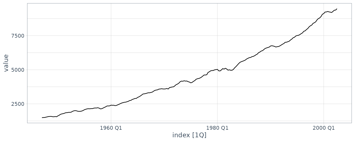
When reports of GNP and similar economic indicators are given, it is often the growth rate that is of interest.

gnp$gnpgr <- c(NA, diff(log(gnp$value)))   
gnp |>
  autoplot(gnpgr) +
  theme_tq()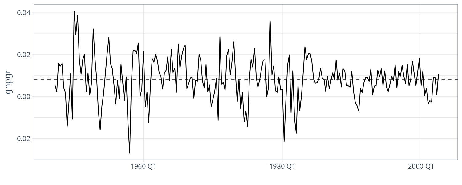

Plotting the ACF/PACF:

\[\begin{aligned} plot_grid( gnp |> ACF(gnpgr) |> autoplot() + geom_line() + ggtitle("ACF") + theme_tq(), gnp |> PACF(gnpgr) |> autoplot() + geom_line() + ggtitle("PACF") + theme_tq(), ncol = 1 ) \end{aligned}\]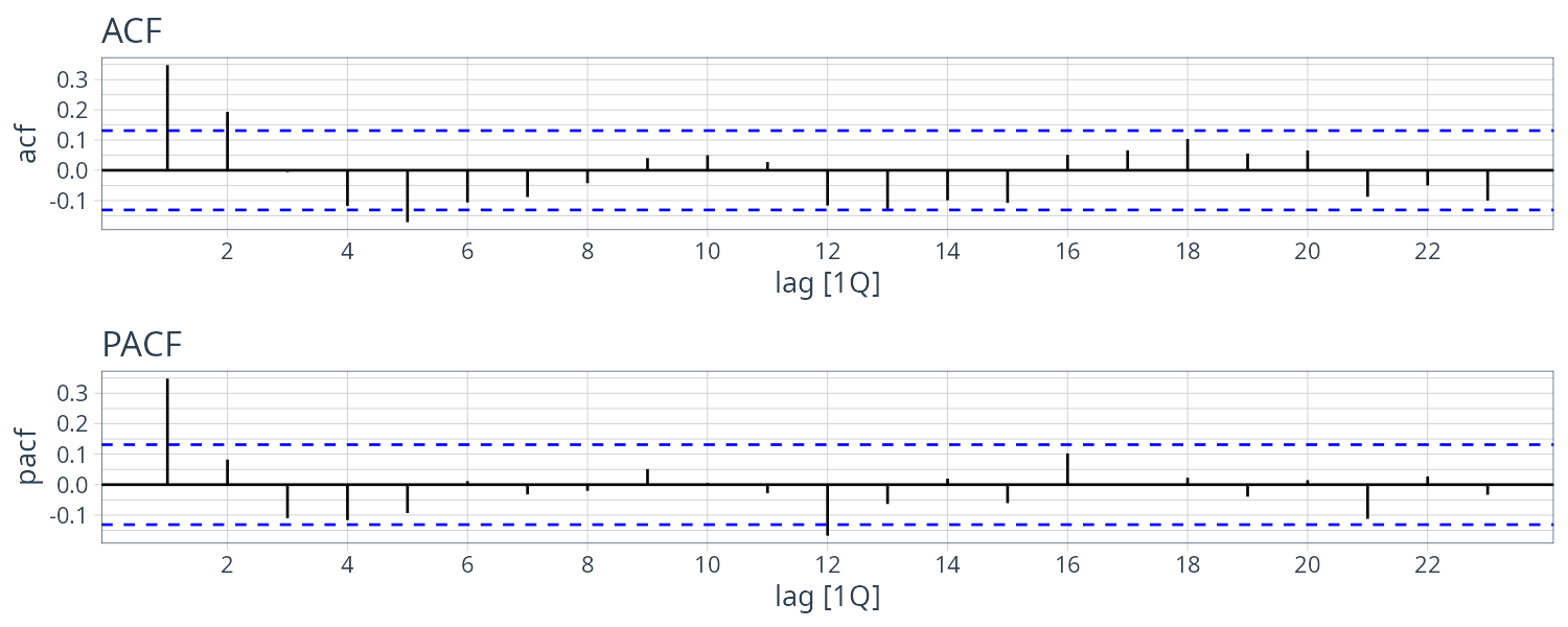

The ACF seem to cut off at lag 2 and PACF is tailing off. This suggests a MA(2) model. Or we could interpret the ACF as tailing off and PACF is cut off at lag 1 which suggests a AR(1) model. We will fit both.

Using MLE to fit the MA(2) model:

fit <- gnp |>
  model(ARIMA(gnpgr ~ 1 + pdq(0, 0, 2) + PDQ(0, 0, 0)))
> tidy(fit)
# A tibble: 3 × 6
  .model                                         term     estimate std.error statistic  p.value
  <chr>                                          <chr>       <dbl>     <dbl>     <dbl>    <dbl>
1 ARIMA(gnpgr ~ 1 + pdq(0, 0, 2) + PDQ(0, 0, 0)) ma1       0.303    0.0654        4.63 6.29e- 6
2 ARIMA(gnpgr ~ 1 + pdq(0, 0, 2) + PDQ(0, 0, 0)) ma2       0.204    0.0644        3.16 1.80e- 3
3 ARIMA(gnpgr ~ 1 + pdq(0, 0, 2) + PDQ(0, 0, 0)) constant  0.00833  0.000955      8.72 6.50e-16      

> sqrt(glance(fit)$sigma2)
      year 
0.00948697 

\[\begin{aligned} \hat{x}_{t} &= 0.008 + 0.303\hat{w}_{t-1} + 0.204\hat{w}_{t-2} + \hat{w}_{t}\\ \hat{\sigma} &= 0.0094 \end{aligned}\]

The estimated AR(1) model is:

fit <- gnp |>
  model(ARIMA(gnpgr ~ 1 + pdq(1, 0, 0) + PDQ(0, 0, 0)))

> tidy(fit)
# A tibble: 2 × 6
  .model                                         term     estimate std.error statistic  p.value
  <chr>                                          <chr>       <dbl>     <dbl>     <dbl>    <dbl>
1 ARIMA(gnpgr ~ 1 + pdq(1, 0, 0) + PDQ(0, 0, 0)) ar1       0.347    0.0627        5.53 9.16e- 8
2 ARIMA(gnpgr ~ 1 + pdq(1, 0, 0) + PDQ(0, 0, 0)) constant  0.00545  0.000638      8.54 2.14e-15

> sqrt(glance(fit)$sigma2)
       year 
0.009523879 

\[\begin{aligned} \hat{x}_{t} &= 0.00545 + 0.347\hat{x}_{t-1} + \hat{w}_{t}\\ &= 0.008(1 - 0.347) + 0.347\hat{x}_{t-1} + \hat{w}_{t} \hat{\sigma} &= 0.0095 \end{aligned}\]

The two models are actually similar. Representing the AR(1) model in causal form (assuming no constant):

\[\begin{aligned} x_{t} &= 0.35x_{t-1} + w_{t}\\ x_{t} &= \sum_{j=0}^{\infty}\psi_{j}w_{t-j}\\ \psi_{j} &= 0.35^{j}\\ \psi_{0} &= 1\\ \psi_{1} &= 0.350\\ \psi_{2} &= 0.123\\ \psi_{3} &= 0.043\\ \vdot\\ x_{t} &\cong 0.35 w_{t-1} + 0.12w_{t-2} + w_{t} \end{aligned}\]

Next we check the diagnostics. We will look at the standardized innovations/residuals:

\[\begin{aligned} e_{t} &= \frac{x_{t} - \hat{x}_{t}^{t-1}}{\sqrt{\hat{P}_{t}^{t-1}}} \end{aligned}\]

If the model fits well, the standardized residuals should behave as an iid sequence with mean 0 and variance 1.

Marginal normality can be accomplished by looking at the histogram of the residuals.

Test of autocorrelations can be done by Ljung–Box–Pierce Q-statistics:

\[\begin{aligned} Q &= n(n+2)\sum_{h=1}^{H}\frac{\hat{p}_{e}^{2}(h)}{n-h}\\ Q &\sim \chi_{H-p-q}^{2} \end{aligned}\]

H is the number of lags and typically \(H=20\). The null hypothesis is no autocorrelations.

fit |>
  gg_tsresiduals()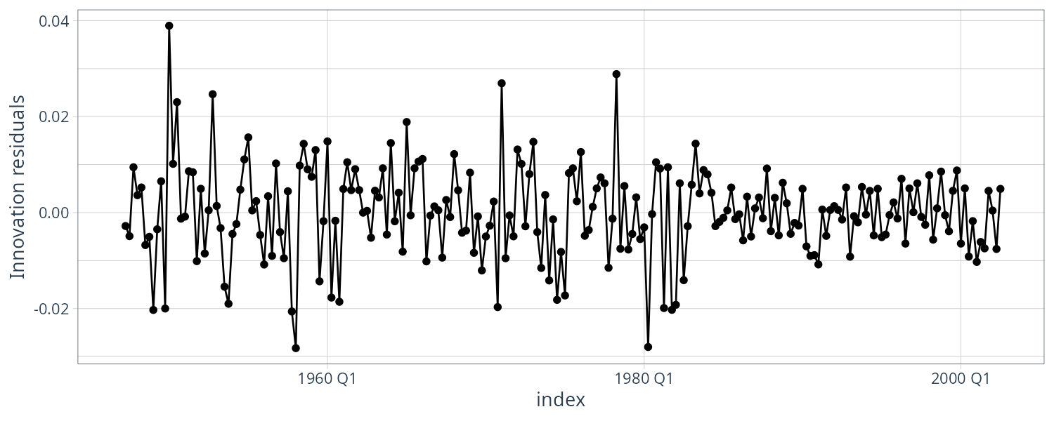   

> augment(fit) |>
  features(.innov, box_pierce, lag = 20)
# A tibble: 1 × 3
  .model                                         bp_stat bp_pvalue
  <chr>                                            <dbl>     <dbl>
1 ARIMA(gnpgr ~ 1 + pdq(1, 0, 0) + PDQ(0, 0, 0))    23.9     0.246     

Model Selection

To choose the final model, we compare the AIC, the AICc, and the BIC of both models:

fit1 <- gnp |>
  model(ARIMA(gnpgr ~ 1 + pdq(0, 0, 2) + PDQ(0, 0, 0)))     

fit2 <- gnp |>
  model(ARIMA(gnpgr ~ 1 + pdq(1, 0, 0) + PDQ(0, 0, 0)))

> glance(fit1) |>
  select(AIC, AICc, BIC)
# A tibble: 1 × 3
     AIC   AICc    BIC
   <dbl>  <dbl>  <dbl>
1 -1432. -1432. -1418.

> glance(fit2) |>
  select(AIC, AICc, BIC)
# A tibble: 1 × 3
     AIC   AICc    BIC
   <dbl>  <dbl>  <dbl>
1 -1431. -1431. -1421.

We can see both AIC and AICc favors MA(2) model but BIC favors AR(1) which is not surprising as BIC favors simpler models.

Regression with Autocorrelated Errors

Consider the regression model:

\[\begin{aligned} y_{t} &= \sum_{j=1}^{r}\beta_{j}z_{tj} + x_{t} \end{aligned}\]

In OLS, \(x_{t}\) is assumed to white noise with covariance function:

\[\begin{aligned} \gamma_{x}(s, t) &= 0\ s\neq t\\ \gamma_{x}(t, t) &= \sigma^{2}\ s = t \end{aligned}\]

If this is not the case, the weighted least squares should be used which we will show below.

In matrix notation:

\[\begin{aligned} \boldsymbol{y} &= Z\boldsymbol{\beta} + \boldsymbol{x}\\ \boldsymbol{y} &= \begin{bmatrix} y_{1} & \cdots & y_{n} \end{bmatrix}^{T}\\ \boldsymbol{x} &= \begin{bmatrix} x_{1} & \cdots & x_{n} \end{bmatrix}^{T}\\ \boldsymbol{\beta} &= \begin{bmatrix} \beta_{1} & \cdots & \beta_{n} \end{bmatrix}^{T}\\ \Gamma &= \{\gamma_{x}(s , t)\} \end{aligned}\]

Then:

\[\begin{aligned} \Gamma^{-\frac{1}{2}}y &= \Gamma^{-\frac{1}{2}}Z\boldsymbol{\beta} + \Gamma^{-\frac{1}{2}}x\\ \boldsymbol{y}^{*} &= Z^{*}\boldsymbol{\beta} + \boldsymbol{\delta}\\ \boldsymbol{y}^{*} &= \Gamma^{-\frac{1}{2}}\boldsymbol{y}\\ Z^{*} &= \Gamma^{-\frac{1}{2}}Z\\ \boldsymbol{\delta} &= \Gamma^{-\frac{1}{2}}\boldsymbol{x} \end{aligned}\]

The weighted estimate of \(\boldsymbol{\beta}\):

\[\begin{aligned} \hat{\boldsymbol{\beta}}_{w} &= (Z^{*T}Z^{*})^{-1}Z^{*T}\boldsymbol{y}^{*}\\ &= (Z^{T}\Gamma^{-1}Z)^{-1}Z^{T}\Gamma^{-1}\boldsymbol{y}\\ \text{var}(\hat{\boldsymbol{\beta}}_{w} &= (Z^{T}\Gamma^{-1}Z)^{-1} \end{aligned}\]

If \(x_{t}\) is white noise, then:

\[\begin{aligned} \Gamma &= \sigma^{2}I \end{aligned}\]

Recall that if we have a AR(p) process, then:

\[\begin{aligned} \phi(B)x_{t} &= w_{t} \end{aligned}\]

Multiplying the regression equation by \(\phi(B)\):

\[\begin{aligned} \phi(B)y_{t} &= \sum_{j=1}^{r}\beta_{j}\phi(B)z_{tj} + \phi(B)x_{t} \end{aligned}\]

Now we are back to the linear regression model where the observations have been transformed:

\[\begin{aligned} \phi(B)y_{t} &= \sum_{j=1}^{r}\beta_{j}\phi(B)z_{tj} + \phi(B)x_{t}\\ y_{t}^{*} &= \sum_{j=1}^{r}\beta_{j}z_{tj}^{*} + w_{t}\\ y_{t}^{*} &= \phi(B)y_{}\\ z_{tj}^{*} &= \phi(B)z_{tj} \end{aligned}\]

We then set up the least squares problem as minimizing the sum of squares error:

\[\begin{aligned} S(\phi, \beta) &= \sum_{t=1}w_{t}^{2}\\ &= \sum_{t=1}^{n}(\phi(B)y_{t} - \sum_{j=1}^{r})\beta_{j}\phi(B)z_{tj})^{2} \end{aligned}\]

Now, if the error is ARMA(p,q) instead of AR(p) then:

\[\begin{aligned} \phi(B)x_{t} &= \theta(B)w_{t}\\ \pi(B)x_{t}&= \theta(B)^{-1}\phi(B) \end{aligned}\]

In this case, the sum of squares error:

\[\begin{aligned} S(\phi, \theta, \beta) &= \sum_{t=1}^{n}w_{t}^{2}\\ &= \sum_{t=1}^{n}(\pi(B)y_{t} - \sum_{j=1}^{r}\beta_{j}\pi(B)z_{tj})^{2} \end{aligned}\]

Typically we do not know the behavior of the noise. So we do the following steps:

• Run an OLS of \(y_{t}\) on \(z_{t1}, \cdots, z_{tr}\)
• Retain the residuals \(\hat{x}_{t} &= y_{t} - \sum_{j=1}^{r}\hat{beta}_{j}z_{tj}\)
• Identify the ARMA mdels for the residuals \(\hat{x}_{t}\)
• Run weighted least squares on the regression model with autocorrelation errors
• Inspect the residuals \(\hat{w}_{t}\) and repeat if necessary

Example: Mortality, Temperature and Pollution

We consider the regression model:

\[\begin{aligned} M_{t} &= \beta_{1} + \beta_{2}t + \beta_{3}T_{t} + \beta_{4}T_{t}^{2} + \beta_{5}P_{t} + x_{t} \end{aligned}\]

Checking the ACF/PACF, we tried using AR(2) model for the residuals:

cmort <- as_tsibble(cmort)
tempr <- as_tsibble(tempr)
part <- as_tsibble(part)

dat <- tsibble(
  t = seq(
    as.Date("1970-01-01"),
    as_date(yearweek("1979 Week 40")),      
    by = "1 week")[1:508],
  cmort = cmort$value,
  tempr = tempr$value,
  part = part$value,
  index = t
) |>
  mutate(
    temp = tempr - mean(tempr),
    temp2 = temp^2,
    trend = 1:nrow(dat)
  )

fit <- lm(
  cmort ~ trend +
    temp +
    temp2 +
    part,
  data = dat
)
dat$resid <- resid(fit)

plot_grid(
  dat |>
    ACF(resid) |>
    autoplot() +
    ggtitle("ACF") +
    theme_tq(),
  dat |>
    PACF(resid) |>
    autoplot() +
    ggtitle("PACF") +
    theme_tq(),
  ncol = 1
)

\[\begin{aligned} x_{t} &= \phi_{1}x_{t-1} + \phi_{2}x_{t-2} + w_{t} \end{aligned}\]

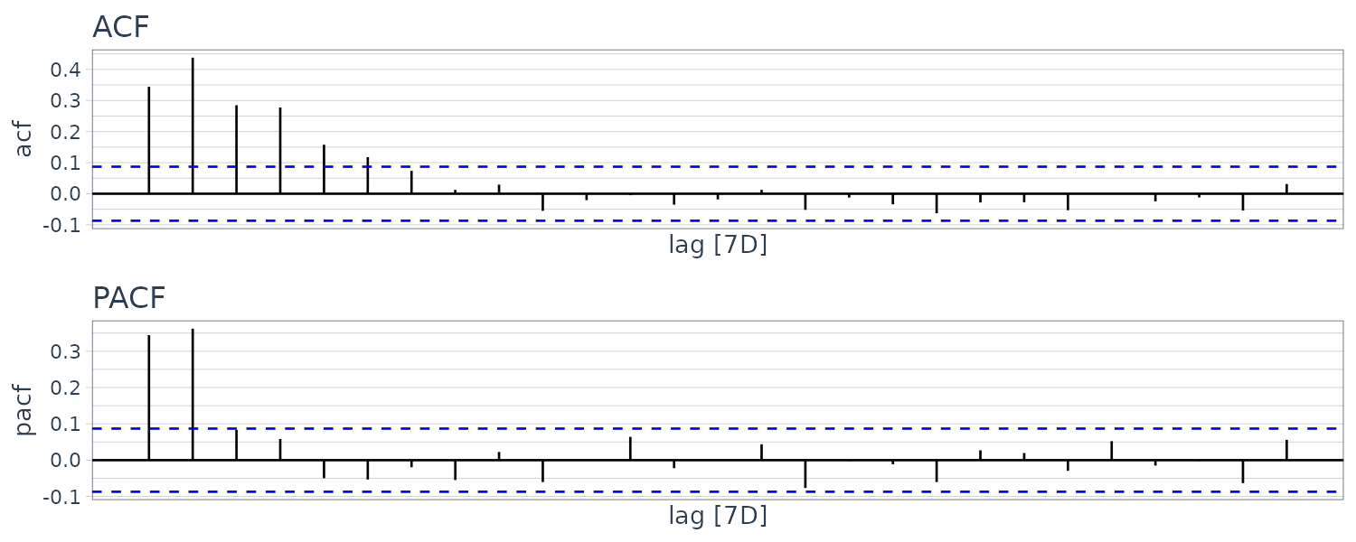
Next we fit a model with AR(2) errors:

fit <- dat |>
  model(
    ARIMA(
      cmort ~ trend +
        temp +
        temp2 +
        part +
        pdq(2, 0, 0) +    
        PDQ(0, 0, 0)
    )
  )
> report(fit)
Series: cmort 
Model: LM w/ ARIMA(2,0,0) errors 

Coefficients:
         ar1     ar2    trend     temp   temp2    part  intercept     
      0.3848  0.4326  -0.0292  -0.0190  0.0154  0.1545    87.6338
s.e.  0.0436  0.0400   0.0081   0.0495  0.0020  0.0272     2.7848

sigma^2 estimated as 26.38:  log likelihood=-1549.04
AIC=3114.07   AICc=3114.36   BIC=3147.92

Checking the residuals again, we see there is no departure from white noise.

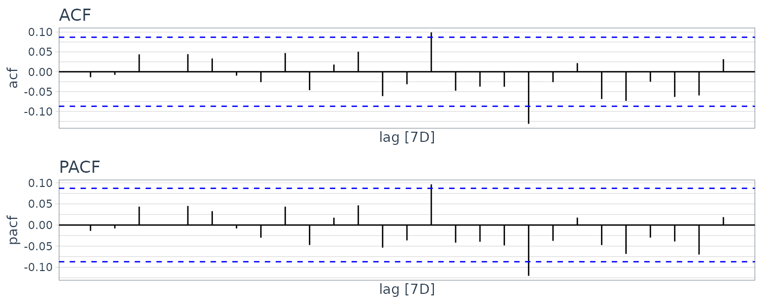
Example: Regression with Lagged Variables

Earlier we fit the following model:

\[\begin{aligned} R_{t} &= \beta_{0} + \beta_{1}S_{t-6} + \beta_{2}D_{t-6} + \beta_{3}D_{t-6}S_{t-6} + w_{t} \end{aligned}\]

dummy <- ifelse(soi$value < 0, 0, 1)

dat <- tsibble(
  t = rec$index,
  rec = rec$value,
  soi = soi$value,
  soiL6 = lag(soi$value, 6),
  dL6 = lag(dummy, 6),
  index = t
)

fit <- lm(rec ~ soiL6 * dL6, data = dat)
dat$resid <- c(rep(NA, 6), resid(fit))

plot_grid(
  dat |>
    ACF(resid) |>
    autoplot() +
    ggtitle("ACF") +
    theme_tq(),
  dat |>
    PACF(resid) |>
    autoplot() +
    ggtitle("PACF") +
    theme_tq(),
  ncol = 1
)

The ACF/PACF indicates an AR(2) model for the noise:

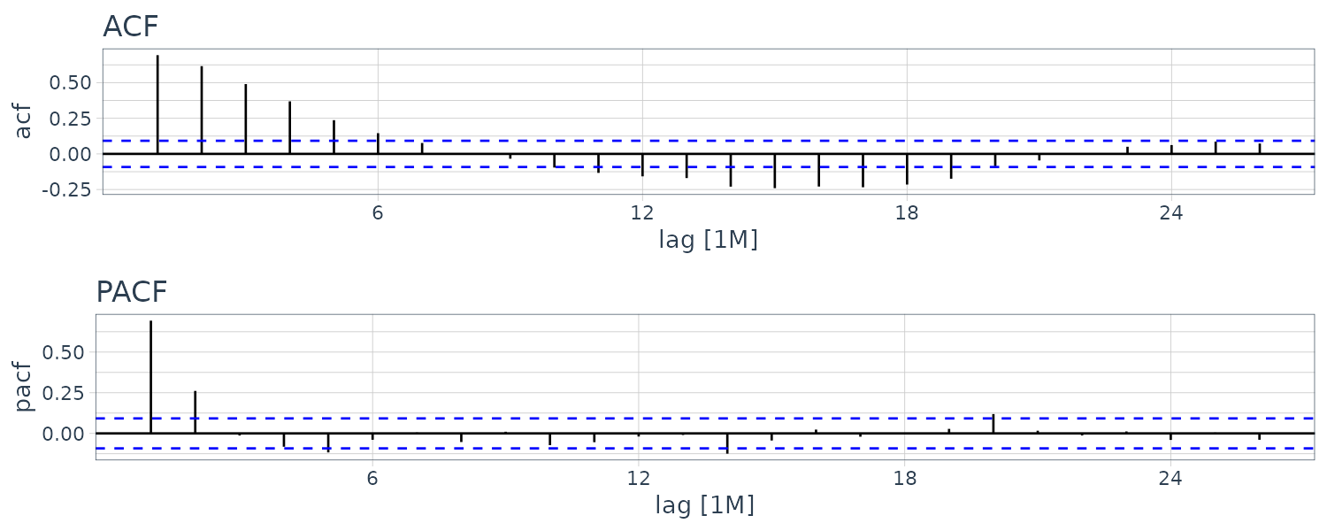
fit <- dat |>
  model(
    ARIMA(
      rec ~ soiL6 * dL6 +
        pdq(2, 0, 0) +
        PDQ(0, 0, 0)
    )
  )

> report(fit)
Series: rec 
Model: LM w/ ARIMA(2,0,0) errors 

Coefficients:
         ar1      ar2   soiL6      dL6  soiL6:dL6  intercept
      1.3624  -0.4703  8.6682  -2.5947   -10.3097    64.8052
s.e.  0.0440   0.0444  2.2204   0.9535     2.8309     4.1125     

sigma^2 estimated as 86.78:  log likelihood=-1633.07
AIC=3280.13   AICc=3280.38   BIC=3308.94

ACF/PACF indicates white noise:

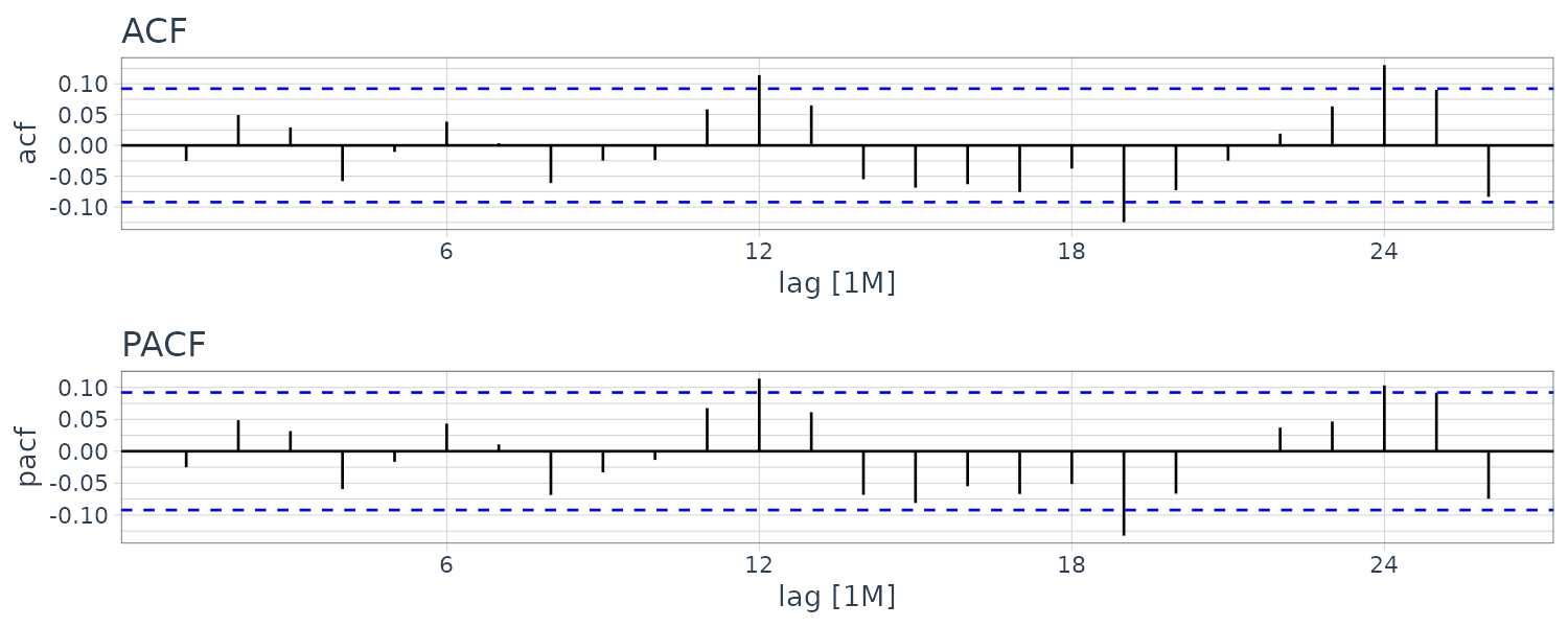
Multiplicative Seasonal ARIMA Models

The pure seasonal ARMA(P, Q) takes the form:

\[\begin{aligned} \Phi_{P}(B^{s})x_{t} &= \Theta_{Q}(B^{S})w_{t}\\ \Phi_{P}(B^{s}) &= 1 - \Phi_{1}B^{S} - \cdots - \Phi_{P}B^{PS}\ \Theta_{Q}(B^{S}) &= 1 + \Theta_{1}B^{S} + \cdots + \Theta_{Q}B^{QS} \end{aligned}\]

\(\Phi_{P}\) is the seasonal autoregressive operator, and \(\Phi_{Q}\) is the seasonal moving average operator. Similarly, the roorts of \(\Phi_{P}(z^{S})\) lie outside the unit circle, and it is invertible only when the roots of \(\Phi_{P}(z^{S})\) lie outside the unit circle.

Example: A Seasonal AR Series

\[\begin{aligned} (1 - \Phi B^{12})x_{t} &= w_{t}\\ x_{t} &= \Phi x_{t-12} + w_{t}\\ |\Phi| < 1 \end{aligned}\]

We simulate 3 years of data with \(\Phi = 0.9\):

set.seed(666)
phi <- c(rep(0, 11), 0.9)
dat <- as_tsibble(
  arima.sim(
    list(order = c(12, 0, 0), ar = phi),     
    n = 37) |>
    ts(freq = 12)
) |>
  rename(
    sAR = value
  )

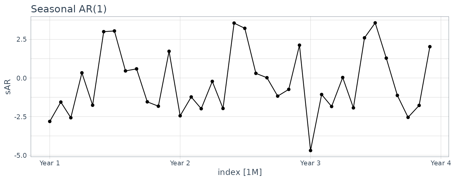
And plotting the ACF/PACF:

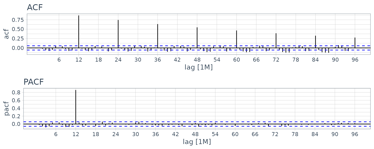
In general, we combine the seasonal and nonseasonal operators into a multiplicative seasonal autoregressive moving average model, \(\text{ARMA}(p, q) \times (P, Q)_{s}\)

\[\begin{aligned} \Phi_{P}(B^{S})\phi(B)x_{t} &= \Theta_{Q}(B^{S})\theta(B)w_{t} \end{aligned}\]

Consider an \(\text{ARMA}(0, 1)\times(1, 0)_{12}\) model:

\[\begin{aligned} x_{t} &= \Phi x_{t-12} + w_{t} + \theta w_{t-1}\\ |\Phi| < 1\\ |\theta| < 1 \end{aligned}\]

Because \(x_{t-12}, w_{t}, w_{t-1}\) are uncorrelated:

\[\begin{aligned} \gamma(0) &= \Phi^{2}\gamma(0) + \sigma_{w}^{2} + \theta^{2}\sigma_{w}^{2}\\ (1 - \Phi^{2})\gamma(0) &= (1 + \theta^{2})\sigma_{w}^{2}\\ \gamma(0) &= \frac{1 + \theta^{2}}{1 - \Phi^{2}}\sigma_{w}^{2} \end{aligned}\]

We can show that:

\[\begin{aligned} E[x_{t}x_{t-h}] &= \Phi E[x_{t-12}x_{t-h}]\\ \gamma(h) &= \Phi\gamma(h-12)\\ \gamma(12h) &= \Phi\gamma(12h - 12)\\ &= \Phi^{h}\gamma(12h - 12h)\\ &= \Phi^{h}\gamma(0)\\ \rho(12h) &= \frac{\gamma(0)}{\gamma(0)}\Phi^{h}\\ &= \Phi^{h} \end{aligned}\]

We can also show that:

\[\begin{aligned} \rho(12h - 1) &= \rho(12h + 1)\\ &= \frac{\theta}{1 + \theta^{2}}\Phi^{h}\\ \rho(h) &= 0\ \text{otherwise} \end{aligned}\]

We can simulate the model with:

\[\begin{aligned} \Phi = 0.8\\ \theta = -0.5 \end{aligned}\]

set.seed(666)
phi <- c(rep(0, 11), 0.8)
dat <- as_tsibble(
  arima.sim(
    list(order = c(12, 0, 1), ar = phi, ma = -0.5),     
    n = 12 * 100
  ) |>
    ts(freq = 12)
)

Or we could directly calculate ACF/PACF in R:

phi <- c(rep(0, 11), .8)     
ACF <- ARMAacf(
  ar = phi,
  ma = -.5,
  50
)
PACF <- ARMAacf(
  ar = phi,
  ma = -.5, 50,
  pacf = TRUE
)

Seasonal Persistence

Seasonal persistence occurs when the process is nearly periodic in the season. For example, monthly temperatures over the years. We can think of average monthly temperature \(x_{t}\):

\[\begin{aligned} x_{t} &= S_{t} + w_{t}\\ S_{t} &= S_{t-12} + \nu_{t} \text{cov}(w_{t}, \nu_{t}) &= 0 \end{aligned}\]

If we subtract the effect of successive years from each other:

\[\begin{aligned} (1 - B^{12})x_{t} &= x_{t} - x_{t-12}\\ S_{t} + w_{t} - S_{t-12} - w_{t-12}\\ &= S_{t-12} + \nu_{t} + w_{t} - S_{t-12} - w_{t-12}\\ &= \nu_{t} + w_{t} - w_{t-12} \end{aligned}\]

This model will be a stationary MA(1)_{12} and ACF will peak only at lag 12. In general, seasonal differencing is needed when the ACF decays slowly at multiples of some season, but is negligible between the periods.

The seasonal difference of order D is defined as:

\[\begin{aligned} \nabla_{s}^{D}x_{t} &= (1 - B^{s})^{D}x_{t} \end{aligned}\]

The multiplicaitve seasonal ARIMA (SARIMA) model \(\text{ARIMA}(p, d, q)\times(P,D,Q)_{S}\) is given by:

\[\begin{aligned} \Phi_{P}(B^{S})\phi(B)\nabla_{S}^{D}\nabla^{d}x_{t} &= \delta + \Theta_{Q}(B^{S})\theta(B)w_{t} \end{aligned}\]

Example: An SARIMA Model

Consider a \(\text{ARIMA}(0,1,1)\times(0,1,1)_{12}\), then with \(\delta=0\):

\[\begin{aligned} \nabla_{12}\nabla x_{t} &= \Theta(B^{12})\theta(B)w_{t}\\ (1 - B^{12})(1 - B)x_{t} &= (1 + \Theta B^{12})(1 + \theta B)w_{t} \end{aligned}\\ (1 - B - B^{12} + b^{13})x_{t} &= (1 + \theta B + \Theta B^{12} + \Theta \theta B^{13})w_{t}\]

Or in difference equation:

\[\begin{aligned} x_{t} &= x_{t-1} + x_{t-12} - x_{t-13} + w_{t} + \theta w_{t-1} + \Theta w_{t-12} + \Theta \theta w_{t-13} \end{aligned}\]

Note that the multiplicative nature of the model implies that the coefficietnt of \(w_{t-13}\) is the result of the product of \(w_{t-1}, w_{t-12}\) rather than a free parameter.

Example: Air Passengers

Consider the dataset AirPassengers. Let’s plot the data and transformed data:

AirPassengers <- as_tsibble(AirPassengers)

AirPassengers <- AirPassengers |>
  rename(x = value) |>
  mutate(
    lx = log(x),
    dlx = c(NA, diff(lx)),
    ddlx = c(rep(NA, 12), diff(dlx, 12))     
  )

plot_grid(
  AirPassengers |>
    autoplot(x) +
    theme_tq(),
  AirPassengers |>
    autoplot(lx) +
    theme_tq(),
  AirPassengers |>
    autoplot(dlx) +
    theme_tq(),
  AirPassengers |>
    autoplot(ddlx) +
    theme_tq(),
  ncol = 1
)

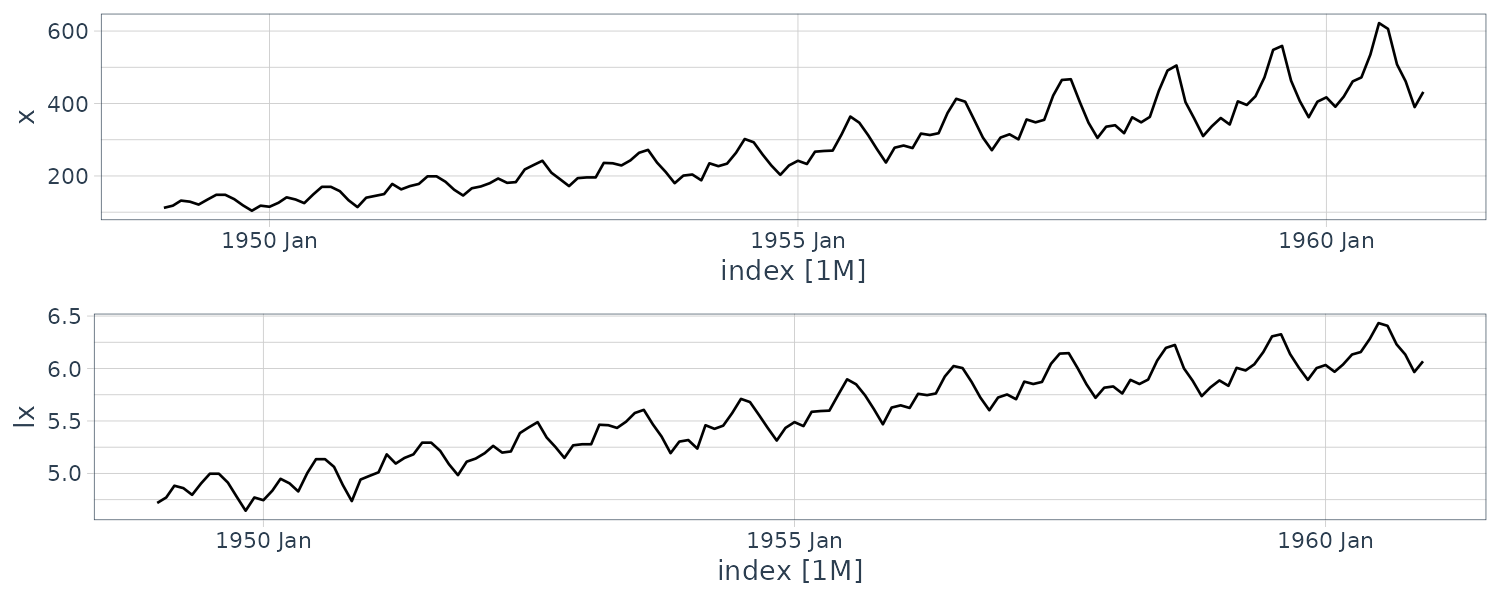
Next we plot the ACF/PACF. For the seasonal component, it appears that the ACF is cutting off at lag 12 and PACF is tailing off at multiple of 12. This suggests a SMA(1).

For the non-seasonal component, the ACF and PACF appears to tail off. This suggests an ARMA(1, 1) model.

We try fitting an \(\text{ARIMA}(1, 1, 1) \times (0, 1,1)_{12}\) model:

fit <- AirPassengers |>
  model(
    ARIMA(
      lx ~ pdq(1, 1, 1) + PDQ(0, 1, 1)
    )
  )

> fit |>
  report()
Series: lx 
Model: ARIMA(1,1,1)(0,1,1)[12] 

Coefficients:
         ar1      ma1     sma1
      0.1960  -0.5784  -0.5643
s.e.  0.2475   0.2132   0.0747

sigma^2 estimated as 0.001375:  log likelihood=244.95     
AIC=-481.9   AICc=-481.58   BIC=-470.4

> fit |>
  tidy()
# A tibble: 3 × 6
  .model                                  term  estimate std.error statistic  p.value
  <chr>                                   <chr>    <dbl>     <dbl>     <dbl>    <dbl>
1 ARIMA(lx ~ pdq(1, 1, 1) + PDQ(0, 1, 1)) ar1      0.196    0.247      0.792 4.30e- 1
2 ARIMA(lx ~ pdq(1, 1, 1) + PDQ(0, 1, 1)) ma1     -0.578    0.213     -2.71  7.57e- 3
3 ARIMA(lx ~ pdq(1, 1, 1) + PDQ(0, 1, 1)) sma1    -0.564    0.0747    -7.55  6.42e-12     

Since the AR1 parameter is not significant, let’s try dropping that and fit \(\text{ARIMA}(0, 1, 1)\times(0, 1, 1)_{12}\) model:

fit <- AirPassengers |>
  model(
    ARIMA(
      lx ~ pdq(0, 1, 1) + PDQ(0, 1, 1)     
    )
  )

> fit |>
  report()
Series: lx 
Model: ARIMA(0,1,1)(0,1,1)[12] 

Coefficients:
          ma1     sma1
      -0.4018  -0.5569
s.e.   0.0896   0.0731

sigma^2 estimated as 0.001371:  log likelihood=244.7     
AIC=-483.4   AICc=-483.21   BIC=-474.77

Finally, weo do aforecast 12 months out:

fit |>
  forecast(h = 12) |>
  autoplot(AirPassengers) +    
  theme_tq()

See Also

References

Shuway H. (2017) Time Series Analysis and Its Applications: With R Examples (Springer Texts in Statistics) 4th ed.