TidyModels
Read PostIn this post we will follow the book Tidy Modeling with R.
Contents:
- Data Analysis Process
- Ames Housing Data
- Splitting Data
- Fitting Model
- Model Workflow
- Recipes
- Metrics
- Comparing Models
- Resampling
- Model Tuning
- Screening Multiple Models
- Dimensionality Reduction
- Encoding Categorical Data
- Explaining Models
- Prediction Quality
- Ensembles of Models
- Inferential Analysis
- See Also
- References
Data Analysis Process
The general phases of data analysis are:
- Exploratory Data Analysis (EDA)
- Feature Engineering
- Model Tuning and Selection
- Model Evaluation
As an example, Kuhn and Johnson use data to model the daily ridership of Chicago’s public train system. These are the hypothetical inner monologues in chronological order:
1) EDA
- The daily ridership values between stations seemed extremely correlated
- Weekday and weekend ridership look very different
- One day in the summer of 2010 has an abnormally large number of riders
- Which stations had the lowest daily ridership values?
2) Feature Engineering
- Dates should at least be encoded as day-of-the-week and year
- Maybe PCA could be used on the correlated predictors to make it easier for the models to use them
- Hourly weather records should probably be averaged into daily measurements
3) Model Fitting
- Let’s start with simple linear regression, K-nearest neighbors, and a boosted decision tree
4) Model Tuning
- How many neighbors should be used?
- Should we run a lot of boosting iterations or just a few?
- How many neighbors seemed to be optimal for these data?
5) Model Evaluation
- Which models have the lowest root mean squared errors?
6) EDA
- Which days were poorly predicted?
7) Model Evaluation
- Variable importance scores indicate that the weather information is not predictive. We’ll drop them from the next set of models.
- It seems like we should add a lot of boosting iterations for that model
8) Feature Engineering
- We need to encode holiday features to improve predictions
9) Model Evaluation
- Let’s drop KNN from the model list
Ames Housing Data
In this section, we’ll look into the Ames housing data set and do exploratory data analysis. The data set contains information on 2,930 properties in Ames.
library(tidymodels)

dim(ames)
> [1] 2930   74
Selecting the first 5 out of 74 columns:
> ames |>
  select(1:5)
# A tibble: 2,930 × 5
   MS_SubClass                         MS_Zoning                Lot_Frontage Lot_Area Street
   <fct>                               <fct>                           <dbl>    <int> <fct>
 1 One_Story_1946_and_Newer_All_Styles Residential_Low_Density           141    31770 Pave
 2 One_Story_1946_and_Newer_All_Styles Residential_High_Density           80    11622 Pave
 3 One_Story_1946_and_Newer_All_Styles Residential_Low_Density            81    14267 Pave
 4 One_Story_1946_and_Newer_All_Styles Residential_Low_Density            93    11160 Pave
 5 Two_Story_1946_and_Newer            Residential_Low_Density            74    13830 Pave
 6 Two_Story_1946_and_Newer            Residential_Low_Density            78     9978 Pave
 7 One_Story_PUD_1946_and_Newer        Residential_Low_Density            41     4920 Pave
 8 One_Story_PUD_1946_and_Newer        Residential_Low_Density            43     5005 Pave
 9 One_Story_PUD_1946_and_Newer        Residential_Low_Density            39     5389 Pave
10 Two_Story_1946_and_Newer            Residential_Low_Density            60     7500 Pave
# ℹ 2,920 more rows
# ℹ Use `print(n = ...)` to see more rowsggplot(
ames,
aes(x = Sale_Price)
) +
geom_histogram(
bins = 50,
col = "white"
)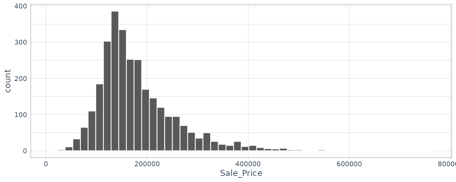
As we can see the data is skew to the right (there are more inexpensive house than super expensive ones). Let’s do a log transformation:
ggplot(
  ames,
  aes(x = Sale_Price)
) +
  geom_histogram(
    bins = 50,
    col = "white"
) |>
scale_x_log10()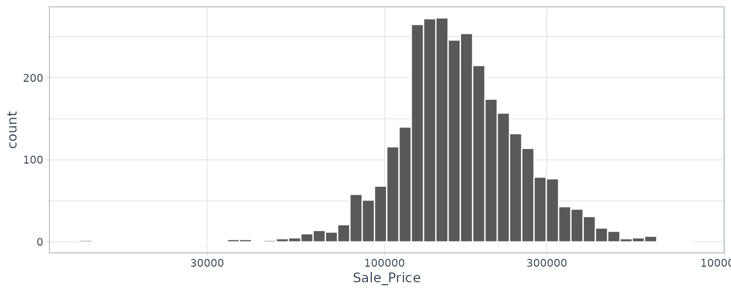
We will add the log transformation as a new outcome column:
ames <- ames |>
  mutate(
    Sale_Price = log10(Sale_Price)
  )
Splitting Data
Splitting the data into 80% training set and 20% test set using random sampling via the rsample package:
set.seed(501)
ames_split <- initial_split(
  ames,
  prop = 0.80
)

> ames_split
<Training/Testing/Total>
<2344/586/2930>
When there is a large class imbalance in classification, it is better to use stratified sampling. The training/test split is conducted separately within each class. For regression problems, the outcome variable can be binned into quartiles, and then stratified sampling can be conducted 4 separate times.
Let’s create the density distribution and quartiles:
sale_dens <- density(
  ames$Sale_Price,
  n = 2^10
) |>
  tidy()

> sale_dens
# A tibble: 1,024 × 2
       x         y
   <dbl>     <dbl>
 1  4.02 0.0000688
 2  4.02 0.0000836
 3  4.02 0.000101
 4  4.02 0.000122
 5  4.03 0.000147
 6  4.03 0.000176
 7  4.03 0.000210
 8  4.03 0.000250
 9  4.03 0.000296
10  4.04 0.000348
# ℹ 1,014 more rows
# ℹ Use `print(n = ...)` to see more rows

quartiles <- quantile(
  ames$Sale_Price,
  probs = c(0.25, 0.50, 0.75)
)

quartiles <- tibble(
  prob = c(0.25, 0.50, 0.75),
  value = unname(quartiles)
)

# linearly interpolate given datapoints
quartiles$y <- approx(
  sale_dens$x,
  sale_dens$y,
  xout = quartiles$value
)$y

> quartiles
# A tibble: 3 × 3
   prob value     y
  <dbl> <dbl> <dbl>
1  0.25  5.11  2.42
2  0.5   5.20  2.36
3  0.75  5.33  1.59
We can graph the quartiles using the following code:
ggplot(
  ames,
  aes(x = Sale_Price)
) +
  geom_line(stat = "density") +
  geom_segment(
    data = quartiles,
    aes(
      x = value, xend = value,
      y = 0, yend = y
    ),
    lty = 2
  ) +
  labs(
    x = "Sale Price (log-10 USD)",
    y = NULL
  ) +
  theme_tq()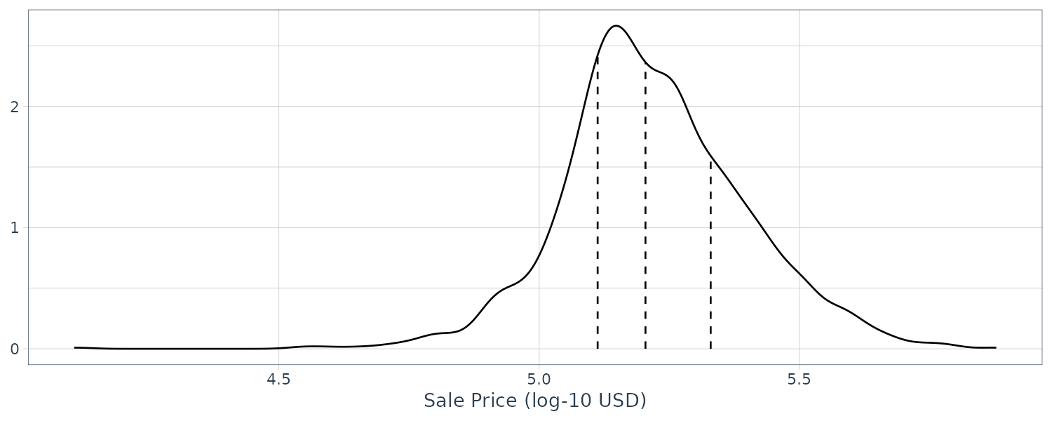
In our Ames case, expensive houses are rarer, so we can use the following stratfied sampling instead:
ames_split <- initial_split(
  ames,
  prop = 0.80,
  strata = Sale_Price
)
Extracting the training and test sets:
ames_train <- training(ames_split)
ames_test <- testing(ames_split)
For time series data, we would use:
initial_time_split(
  ames,
  prop = 0.80
)
It assumes that the data have been presorted in choronological order.
Fitting Model
We are going to fit models using parsnip:
lm_model <- linear_reg() |>
  set_engine("lm")

lm_form_fit <- lm_model |>
  fit(
    Sale_Price ~ Longitude + Latitude,
    data = ames_train
  )

> lm_form_fit
parsnip model object

Call:
stats::lm(formula = Sale_Price ~ Longitude + Latitude, data = data)

Coefficients:
(Intercept)    Longitude     Latitude
   -308.415       -2.074        2.842

lm_xy_fit <- lm_model |>
  fit_xy(
    x = ames_train |>
      select(Longitude, Latitude),
    y = ames_train |>
      pull(Sale_Price)
  )

> lm_xy_fit
parsnip model object

Call:
stats::lm(formula = ..y ~ ., data = data)

Coefficients:
(Intercept)    Longitude     Latitude
   -294.660       -1.984        2.714
Parsnip enables a consistent model interface for different packages. For example, using the ranger package:
rand_fit <- rand_forest(
  trees = 1000,
  min_n = 5
) |>
  set_engine("ranger") |>
  set_mode("regression")

> rand_fit |>
  translate()

Random Forest Model Specification (regression)

Main Arguments:
  trees = 1000
  min_n = 5

Computational engine: ranger

Model fit template:
ranger::ranger(x = missing_arg(), y = missing_arg(), weights = missing_arg(),
    num.trees = 1000, min.node.size = min_rows(~5, x), num.threads = 1,
    verbose = FALSE, seed = sample.int(10^5, 1))
Using Model Results
fit <- lm_form_fit |>
   extract_fit_engine()

> fit
Call:
stats::lm(formula = ..y ~ ., data = data)

Coefficients:
(Intercept)    Longitude     Latitude
   -294.660       -1.984        2.714


> summary(fit)
Call:
stats::lm(formula = ..y ~ ., data = data)

Residuals:
     Min       1Q   Median       3Q      Max
-1.03203 -0.09707 -0.01845  0.09851  0.51067

Coefficients:
             Estimate Std. Error t value            Pr(>|t|)
(Intercept) -294.6600    14.5168  -20.30 <0.0000000000000002 ***
Longitude     -1.9839     0.1309  -15.16 <0.0000000000000002 ***
Latitude       2.7145     0.1792   15.15 <0.0000000000000002 ***
---
Signif. codes:  0 ‘***’ 0.001 ‘**’ 0.01 ‘*’ 0.05 ‘.’ 0.1 ‘ ’ 1

Residual standard error: 0.1613 on 2339 degrees of freedom
Multiple R-squared:  0.1613,	Adjusted R-squared:  0.1606
F-statistic:   225 on 2 and 2339 DF,  p-value: < 0.00000000000000022
The broom::tidy() function converts the result into tibble:
> tidy(fit)
# A tibble: 3 × 5
  term        estimate std.error statistic  p.value
  <chr>          <dbl>     <dbl>     <dbl>    <dbl>
1 (Intercept)  -295.      14.5       -20.3 1.68e-84
2 Longitude      -1.98     0.131     -15.2 1.37e-49
3 Latitude        2.71     0.179      15.1 1.59e-49
Predictions
ames_test_small <- ames_test |>
  slice(1:5)

> predict(
  lm_form_fit,
  new_data = ames_test_small
)
# A tibble: 5 × 1
  .pred
  <dbl>
1  5.22
2  5.27
3  5.27
4  5.24
5  5.24
Merging the results from multiple call to predict:
> ames_test_small |>
  select(Sale_Price) |>
  bind_cols(
    predict(
      lm_form_fit,
      ames_test_small
    )
  ) |>
  bind_cols(
    predict(
      lm_form_fit,
      ames_test_small,
      type = "pred_int"
    )
  )
# A tibble: 5 × 4
  Sale_Price .pred .pred_lower .pred_upper
       <dbl> <dbl>       <dbl>       <dbl>
1       5.39  5.22        4.90        5.53
2       5.28  5.27        4.96        5.59
3       5.27  5.27        4.95        5.59
4       5.06  5.24        4.92        5.56
5       5.26  5.24        4.92        5.56
Let’s fit the same data using random forest. The steps are the same:
tree_model <- decision_tree(min_n = 2) |>
  set_engine("rpart") |>
  set_mode("regression")

tree_fit <- tree_model |>
  fit(
    Sale_Price ~ Longitude + Latitude,
    data = ames_train
  )

ames_test_small |>
  select(Sale_Price) |>
  bind_cols(
    predict(
      tree_fit,
      ames_test_small
    )
  )
Model Workflow
Workflow is similar to pipelines in mlr3.
lm_wflow <- workflow() |>
  add_model(
    linear_reg() |>
      set_engine("lm")
  ) |>
  add_formula(Sale_Price ~ Longitude + Latitude)

> lm_wflow
══ Workflow ══════════════════════════════════════
Preprocessor: Formula
Model: linear_reg()

── Preprocessor ──────────────────────────────────
Sale_Price ~ Longitude + Latitude

── Model ─────────────────────────────────────────
Linear Regression Model Specification (regression)

Computational engine: lm

lm_fit <- fit(lm_wflow, ames_train)

> predict(
  lm_fit,
  ames_test |> slice(1:3)
)
# A tibble: 3 × 1
  .pred
  <dbl>
1  5.22
2  5.21
3  5.28
Workflow can be updated as well:
lm_fit |>
  update_formula(Sale_Price ~ Longitude)
Or adding formulas:
lm_wflow <- lm_wflow |>
  remove_formula() |>
  add_variables(
    outcome = Sale_Price,
    predictors = c(
      Longitude,
      Latitude
    )
  )
And using general selectors:
predictors = c(ends_with("tude"))
predictors = everything()

lm_wflow <- lm_wflow |>
  remove_formula() |>
  add_variables(
    outcome = Sale_Price,
    predictors = predictors
  )
Special Formulas and Inline Functions
Some models use extended formulas that base R functions cannot parse or execute. To get around this problem is to first add the variables and the supplementary model formula afterwards:
library(lme4)
library(multilevelmod)

data(Orthodont, package = "nlme")

multilevel_spec <- linear_reg() |>
  set_engine("lmer")

multilevel_workflow <- workflow() |>
  add_variables(
    outcome = distance,
    predictors = c(
      Sex, age,
      Subject
    )
  ) |>
  add_model(
    multilevel_spec,
    formula = distance ~ Sex + (age | Subject)
  )

multilevel_fit <- fit(
  multilevel_workflow,
  data = Orthodont
)

> multilevel_fit
══ Workflow [trained] ══════════════════════════
Preprocessor: Variables
Model: linear_reg()

── Preprocessor ────────────────────────────────
Outcomes: distance
Predictors: c(Sex, age, Subject)

── Model ───────────────────────────────────────
Linear mixed model fit by REML ['lmerMod']
Formula: distance ~ Sex + (age | Subject)
   Data: data
REML criterion at convergence: 471.1635
Random effects:
 Groups   Name        Std.Dev. Corr
 Subject  (Intercept) 7.3912
          age         0.6943   -0.97
 Residual             1.3100
Number of obs: 108, groups:  Subject, 27
Fixed Effects:
(Intercept)    SexFemale
     24.517       -2.145
And using strata() function from the survival package for survival analysis:
library(censored)

parametric_spec <- survival_reg()

parametric_workflow <- workflow() |>
  add_variables(
    outcome = c(fustat, futime),
    predictors = c(
      age,
      rx
    )
  ) |>
  add_model(
    parametric_spec,
    formula = Surv(futime, fustat) ~ age + strata(rx)
  )

parametric_fit <- fit(
  parametric_workflow,
  data = ovarian
)

> parametric_fit
══ Workflow [trained] ═══════════════════════════════════════════════
Preprocessor: Variables
Model: survival_reg()

── Preprocessor ─────────────────────────────────────────────────────
Outcomes: c(fustat, futime)
Predictors: c(age, rx)

── Model ────────────────────────────────────────────────────────────
Call:
survival::survreg(formula = Surv(futime, fustat) ~ age + strata(rx),
    data = data, model = TRUE)

Coefficients:
(Intercept)         age
 12.8734120  -0.1033569

Scale:
     rx=1      rx=2
0.7695509 0.4703602

Loglik(model)= -89.4   Loglik(intercept only)= -97.1
	Chisq= 15.36 on 1 degrees of freedom, p= 0.0000888
n= 26
Creating Multiple Workflows at Once
We can create a set of formulas:
location <- list(
  longitude = Sale_Price ~ Longitude,
  latitude = Sale_Price ~ Latitude,
  coords = Sale_Price ~ Longitude + Latitude,
  neighborhood = Sale_Price ~ Neighborhood
)
These representations can be crossed with one or more models (in this case lm and glm):
library(workflowsets)
location_models <- workflow_set(
  preproc = location,
  models = list(
    lm = lm_model,
    glm = glm_model
  )
)

> location_models
# A workflow set/tibble: 8 × 4
  wflow_id         info             option    result
  <chr>            <list>           <list>    <list>
1 longitude_lm     <tibble [1 × 4]> <opts[0]> <list [0]>
2 longitude_glm    <tibble [1 × 4]> <opts[0]> <list [0]>
3 latitude_lm      <tibble [1 × 4]> <opts[0]> <list [0]>
4 latitude_glm     <tibble [1 × 4]> <opts[0]> <list [0]>
5 coords_lm        <tibble [1 × 4]> <opts[0]> <list [0]>
6 coords_glm       <tibble [1 × 4]> <opts[0]> <list [0]>
7 neighborhood_lm  <tibble [1 × 4]> <opts[0]> <list [0]>
8 neighborhood_glm <tibble [1 × 4]> <opts[0]> <list [0]>
And extract a particular model based on id:
extract_workflow(
  location_models,
  id = "coords_lm"
)
The columns option and result are populated with specific type of objects that result from resampling.
For now we fit each models by using map():
location_models <- location_models |>
  mutate(
    fit = map(
      info,
      ~ fit(.x$workflow[[1]], ames_train)
    )
  )

> location_models
# A workflow set/tibble: 8 × 5
  wflow_id         info             option    result     fit
  <chr>            <list>           <list>    <list>     <list>
1 longitude_lm     <tibble [1 × 4]> <opts[0]> <list [0]> <workflow>
2 longitude_glm    <tibble [1 × 4]> <opts[0]> <list [0]> <workflow>
3 latitude_lm      <tibble [1 × 4]> <opts[0]> <list [0]> <workflow>
4 latitude_glm     <tibble [1 × 4]> <opts[0]> <list [0]> <workflow>
5 coords_lm        <tibble [1 × 4]> <opts[0]> <list [0]> <workflow>
6 coords_glm       <tibble [1 × 4]> <opts[0]> <list [0]> <workflow>
7 neighborhood_lm  <tibble [1 × 4]> <opts[0]> <list [0]> <workflow>
8 neighborhood_glm <tibble [1 × 4]> <opts[0]> <list [0]> <workflow>
Evaluating the Test Set
To test on the test set, we could invoke the convenience function last_fit() to fit on the training set and evaluate it on the test set:
final_lm_res <- last_fit(
  lm_wflow,
  ames_split
)

> final_lm_res
# Resampling results
# Manual resampling
# A tibble: 1 × 6
  splits             id               .metrics         .notes           .predictions .workflow
  <list>             <chr>            <list>           <list>           <list>       <list>
1 <split [2342/588]> train/test split <tibble [2 × 4]> <tibble [0 × 3]> <tibble>     <workflow>
The .workflow column contains the fitted workflow and can be extracted:
fitted_lm_wflow <- extract_workflow(final_lm_res)

> fitted_lm_wflow
══ Workflow [trained] ═══════════════════
Preprocessor: Formula
Model: linear_reg()

── Preprocessor ─────────────────────────
Sale_Price ~ Longitude + Latitude

── Model ────────────────────────────────

Call:
stats::lm(formula = ..y ~ ., data = data)

Coefficients:
(Intercept)    Longitude     Latitude
   -308.618       -2.083        2.826
And the performance metrics and predictions:
> collect_metrics(final_lm_res)
# A tibble: 2 × 4
  .metric .estimator .estimate .config
  <chr>   <chr>          <dbl> <chr>
1 rmse    standard       0.160 Preprocessor1_Model1
2 rsq     standard       0.176 Preprocessor1_Model1

> collect_predictions(final_lm_res)
# A tibble: 588 × 5
   id               .pred  .row Sale_Price .config
   <chr>            <dbl> <int>      <dbl> <chr>
 1 train/test split  5.29     5       5.28 Preprocessor1_Model1
 2 train/test split  5.24    19       5.15 Preprocessor1_Model1
 3 train/test split  5.26    23       5.33 Preprocessor1_Model1
 4 train/test split  5.24    30       4.98 Preprocessor1_Model1
 5 train/test split  5.32    38       5.49 Preprocessor1_Model1
 6 train/test split  5.32    41       5.34 Preprocessor1_Model1
 7 train/test split  5.30    53       5.20 Preprocessor1_Model1
 8 train/test split  5.30    60       5.52 Preprocessor1_Model1
 9 train/test split  5.29    61       5.55 Preprocessor1_Model1
10 train/test split  5.29    65       5.34 Preprocessor1_Model1
# ℹ 578 more rows
# ℹ Use `print(n = ...)` to see more rows
Recipes
Feature engineering includes transformations and encoding of data. The recipes package can be used to combine different feature engineering and preprocessing tasks into a single object and then apply transformation to it.
Encoding Qualitative Data in a Numeric Format
step_unknown() can be used to change missing values to a dedicated factor level.
step_novel() can allocate a new level that are not encountered in training data.
step_other() can be used to analyze the frequencies of the factor levels and convert infrequently occurring values to a level of “other”, with a specified threshold.
step_dummy() creates dummy variables and has a recipe naming convention.
There are other formats such as Feature Hashing and Effects/Likelihood encodings that we shall cover later.
For interaction, in the ames example, step_interact(~ Gr_Liv_Area:startswith(“Bldg_Type_”)) make dummy variables and form the interactions. In this case, an example a interaction column is Gr_Liv_Area_x_Bldg_Type_Duplex.
Let’s create a recipe that:
- log transformed “Gr_Liv_Area”
- create dummy variables for all nominal predictors
- lumping the bottom 1% of neighborhoods in terms of counts into “other” level
- interaction between Gr_Liv_Area x Bldg_Type
- spline for Latitutde
simple_ames <- recipe(
  Sale_Price ~ Neighborhood +
    Gr_Liv_Area +
    Year_Built +
    Bldg_Type +
    Latitude,
  data = ames_train
) |>
  step_log(
    Gr_Liv_Area,
    base = 10
  ) |>
  step_other(
    Neighborhood,
    threshold = 0.01
  ) |>
  step_dummy(
    all_nominal_predictors()
  ) |>
  step_interact(
    ~ Gr_Liv_Area:starts_with("Bldg_Type_")
  ) |>
  step_ns(
    Latitude,
    deg_free = 20
  )

> simple_ames
── Recipe ─────────────────────────────────────────────────

── Inputs
Number of variables by role
outcome:   1
predictor: 5

── Operations
• Log transformation on: Gr_Liv_Area
• Collapsing factor levels for: Neighborhood
• Dummy variables from: all_nominal_predictors()
• Interactions with: Gr_Liv_Area:starts_with("Bldg_Type_")
• Natural splines on: Latitude
Adding reciple to workflow:
lm_wflow <- workflow() |>
  add_model(
    linear_reg() |>
      set_engine("lm")
  ) |>
  add_recipe(simple_ames)

> lm_wflow
══ Workflow ══════════════════════════════════════════════
Preprocessor: Recipe
Model: linear_reg()

── Preprocessor ──────────────────────────────────────────
5 Recipe Steps

• step_log()
• step_dummy()
• step_dummy()
• step_interact()
• step_ns()

── Model ─────────────────────────────────────────────────
Linear Regression Model Specification (regression)

Computational engine: lm

lm_fit <- fit(lm_wflow, ames_train)

> predict(lm_fit, ames_test)
# A tibble: 588 × 1
   .pred
   <dbl>
 1  5.26
 2  5.09
 3  5.40
 4  5.26
 5  5.21
 6  5.49
 7  5.35
 8  5.14
 9  5.11
10  5.14
# ℹ 578 more rows
# ℹ Use `print(n = ...)` to see more rows
Extracting fitted parsnip object:
lm_fit |>
  extract_fit_parsnip() |>
  tidy() |>
  print(n = 53)

# A tibble: 53 × 5
   term                                                 estimate std.error statistic   p.value
   <chr>                                                   <dbl>     <dbl>     <dbl>     <dbl>
 1 (Intercept)                                          -0.466    0.275     -1.69    9.09e-  2
 2 Gr_Liv_Area                                           0.630    0.0152    41.4     6.75e-280
 3 Year_Built                                            0.00193  0.000131  14.7     4.70e- 47
 4 Neighborhood_College_Creek                            0.106    0.0183     5.83    6.37e-  9
 5 Neighborhood_Old_Town                                -0.0461   0.0117    -3.93    8.62e-  5
 6 Neighborhood_Edwards                                  0.0175   0.0169     1.03    3.01e-  1
 7 Neighborhood_Somerset                                 0.0517   0.0113     4.57    5.14e-  6
 8 Neighborhood_Northridge_Heights                       0.162    0.0289     5.60    2.40e-  8
 9 Neighborhood_Gilbert                                  0.00494  0.0288     0.172   8.64e-  1
10 Neighborhood_Sawyer                                  -0.00145  0.0116    -0.124   9.01e-  1
11 Neighborhood_Northwest_Ames                           0.00464  0.00990    0.468   6.40e-  1
12 Neighborhood_Sawyer_West                             -0.00872  0.0120    -0.727   4.67e-  1
13 Neighborhood_Mitchell                                -0.137    0.0673    -2.04    4.18e-  2
14 Neighborhood_Brookside                               -0.0201   0.0134    -1.50    1.33e-  1
15 Neighborhood_Crawford                                 0.181    0.0186     9.71    7.04e- 22
16 Neighborhood_Iowa_DOT_and_Rail_Road                   0.00723  0.0192     0.377   7.06e-  1
17 Neighborhood_Timberland                              -0.0873   0.0643    -1.36    1.75e-  1
18 Neighborhood_Northridge                               0.0899   0.0141     6.39    2.00e- 10
19 Neighborhood_Stone_Brook                              0.177    0.0332     5.34    1.03e-  7
20 Neighborhood_South_and_West_of_Iowa_State_University  0.0563   0.0205     2.74    6.13e-  3
21 Neighborhood_Clear_Creek                              0.0559   0.0180     3.11    1.88e-  3
22 Neighborhood_Meadow_Village                          -0.285    0.0716    -3.98    7.01e-  5
23 Neighborhood_Briardale                               -0.0955   0.0222    -4.31    1.70e-  5
24 Neighborhood_Bloomington_Heights                      0.0381   0.0352     1.08    2.79e-  1
25 Neighborhood_other                                    0.0732   0.0134     5.46    5.27e-  8
26 Bldg_Type_TwoFmCon                                    0.463    0.250      1.85    6.38e-  2
27 Bldg_Type_Duplex                                      0.521    0.212      2.46    1.41e-  2
28 Bldg_Type_Twnhs                                       1.18     0.277      4.27    2.08e-  5
29 Bldg_Type_TwnhsE                                      0.00198  0.208      0.00949 9.92e-  1
30 Gr_Liv_Area_x_Bldg_Type_TwoFmCon                     -0.156    0.0788    -1.98    4.83e-  2
31 Gr_Liv_Area_x_Bldg_Type_Duplex                       -0.194    0.0662    -2.92    3.48e-  3
32 Gr_Liv_Area_x_Bldg_Type_Twnhs                        -0.406    0.0886    -4.58    4.89e-  6
33 Gr_Liv_Area_x_Bldg_Type_TwnhsE                       -0.0110   0.0668    -0.164   8.70e-  1
34 Latitude_ns_01                                       -0.238    0.0841    -2.82    4.77e-  3
35 Latitude_ns_02                                       -0.205    0.0667    -3.08    2.10e-  3
36 Latitude_ns_03                                       -0.185    0.0688    -2.68    7.34e-  3
37 Latitude_ns_04                                       -0.208    0.0697    -2.99    2.80e-  3
38 Latitude_ns_05                                       -0.195    0.0692    -2.82    4.82e-  3
39 Latitude_ns_06                                       -0.0298   0.0695    -0.429   6.68e-  1
40 Latitude_ns_07                                       -0.0989   0.0680    -1.45    1.46e-  1
41 Latitude_ns_08                                       -0.106    0.0684    -1.54    1.23e-  1
42 Latitude_ns_09                                       -0.114    0.0675    -1.69    9.10e-  2
43 Latitude_ns_10                                       -0.129    0.0672    -1.92    5.54e-  2
44 Latitude_ns_11                                       -0.0804   0.0690    -1.17    2.44e-  1
45 Latitude_ns_12                                       -0.0999   0.0677    -1.47    1.40e-  1
46 Latitude_ns_13                                       -0.107    0.0679    -1.58    1.15e-  1
47 Latitude_ns_14                                       -0.141    0.0670    -2.11    3.53e-  2
48 Latitude_ns_15                                       -0.0798   0.0682    -1.17    2.42e-  1
49 Latitude_ns_16                                       -0.0863   0.0680    -1.27    2.04e-  1
50 Latitude_ns_17                                       -0.180    0.0779    -2.31    2.10e-  2
51 Latitude_ns_18                                       -0.167    0.0750    -2.23    2.58e-  2
52 Latitude_ns_19                                        0.00372  0.0744     0.0501  9.60e-  1
53 Latitude_ns_20                                       -0.178    0.0818    -2.18    2.94e-  2
It is possible to call the tidy() function on a specific step based on the number identifier:
estimated_recipe <- lm_fit |>
  extract_recipe(estimated = TRUE)

> tidy(estimated_recipe, number = 1)
# A tibble: 1 × 3
  terms        base id
  <chr>       <dbl> <chr>
1 Gr_Liv_Area    10 log_kpCTV

> tidy(estimated_recipe, number = 2)
# A tibble: 22 × 3
   terms        retained           id
   <chr>        <chr>              <chr>
 1 Neighborhood North_Ames         other_GmUzK
 2 Neighborhood College_Creek      other_GmUzK
 3 Neighborhood Old_Town           other_GmUzK
 4 Neighborhood Edwards            other_GmUzK
 5 Neighborhood Somerset           other_GmUzK
 6 Neighborhood Northridge_Heights other_GmUzK
 7 Neighborhood Gilbert            other_GmUzK
 8 Neighborhood Sawyer             other_GmUzK
 9 Neighborhood Northwest_Ames     other_GmUzK
10 Neighborhood Sawyer_West        other_GmUzK
# ℹ 12 more rows
# ℹ Use `print(n = ...)` to see more rows

> tidy(estimated_recipe, number = 3)
# A tibble: 26 × 3
   terms        columns            id
   <chr>        <chr>              <chr>
 1 Neighborhood College_Creek      dummy_cPTAb
 2 Neighborhood Old_Town           dummy_cPTAb
 3 Neighborhood Edwards            dummy_cPTAb
 4 Neighborhood Somerset           dummy_cPTAb
 5 Neighborhood Northridge_Heights dummy_cPTAb
 6 Neighborhood Gilbert            dummy_cPTAb
 7 Neighborhood Sawyer             dummy_cPTAb
 8 Neighborhood Northwest_Ames     dummy_cPTAb
 9 Neighborhood Sawyer_West        dummy_cPTAb
10 Neighborhood Mitchell           dummy_cPTAb
# ℹ 16 more rows
# ℹ Use `print(n = ...)` to see more rows

> tidy(estimated_recipe, number = 4)
# A tibble: 4 × 2
  terms                          id
  <chr>                          <chr>
1 Gr_Liv_Area:Bldg_Type_TwoFmCon interact_9BGw4
2 Gr_Liv_Area:Bldg_Type_Duplex   interact_9BGw4
3 Gr_Liv_Area:Bldg_Type_Twnhs    interact_9BGw4
4 Gr_Liv_Area:Bldg_Type_TwnhsE   interact_9BGw4

> tidy(estimated_recipe, number = 5)
# A tibble: 1 × 2
  terms    id
  <chr>    <chr>
1 Latitude ns_23xDA
Interaction
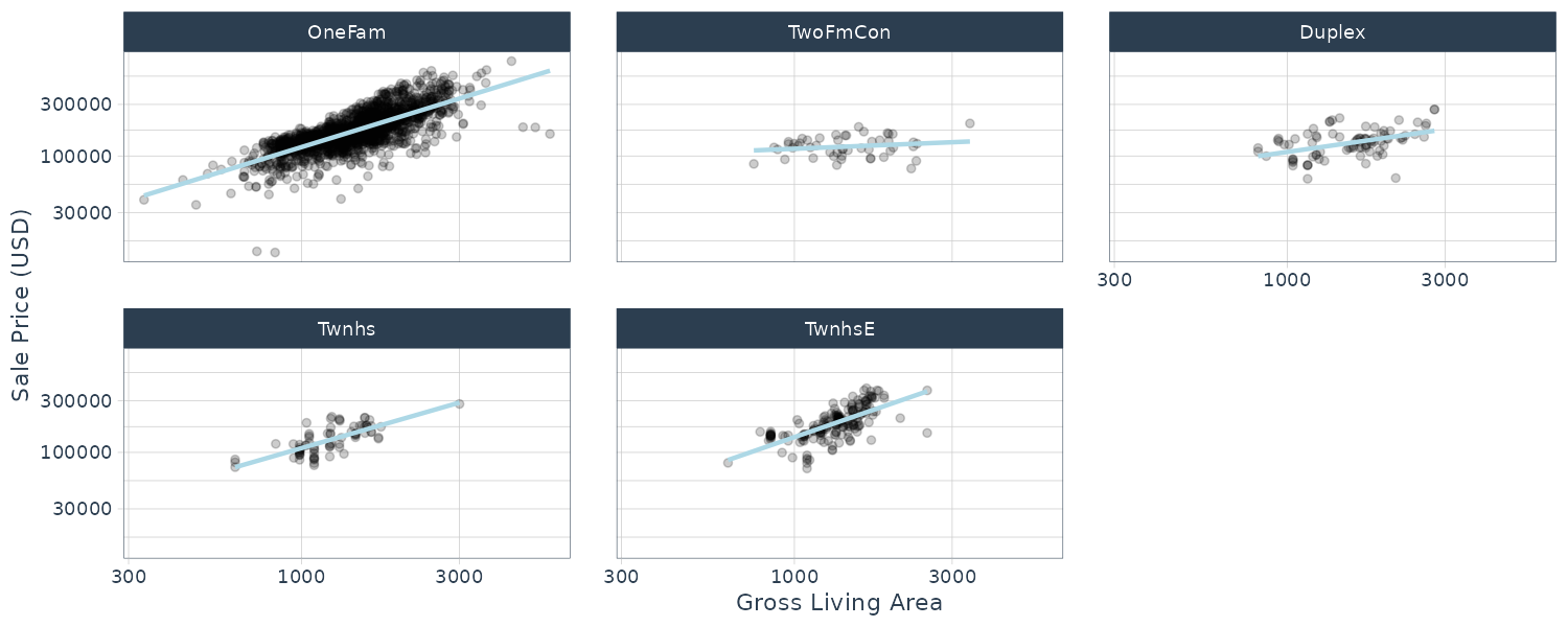
Let us investigate deeper the interaction between Gr_Liv_area x Bldg_Type. By plotting Sale_Price vs Gr_Liv_Area and separate out by Bldg_Type, we can see a difference in the slopes:
ggplot(
  ames_train,
  aes(
    x = Gr_Liv_Area,
    y = 10^Sale_Price
  )
) +
  geom_point(alpha = .2) +
  facet_wrap(~Bldg_Type) +
  geom_smooth(
    method = lm,
    formula = y ~ x,
    se = FALSE,
    color = "lightblue"
  ) +
  scale_x_log10() +
  scale_y_log10() +
  labs(
    x = "Gross Living Area",
    y = "Sale Price (USD)"
  )
Spline
The relationship between SalePrice and Latitude is essentially nonlinear. Latitude is similar to Neighborhood in the sense that both variables are trying to capture the variation in price from the variation of location but in different ways.
The following code graphs different degrees of freedom (# of knots across latitude) and df of 20 (we will tune this parameter later) looks reasonable:
library(splines)
library(patchwork)

plot_smoother <- function(deg_free) {
  ggplot(
    ames_train,
    aes(x = Latitude, y = Sale_Price)
  ) +
    geom_point(alpha = .2) +
    scale_y_log10() +
    geom_smooth(
      method = lm,
      formula = y ~ ns(x, df = deg_free),
      color = "lightblue",
      se = FALSE
    ) +
    labs(
      title = paste(deg_free, "Spline Terms"),
      y = "Sale Price (USD)"
    )
}

(plot_smoother(2) + plot_smoother(5)) /
  (plot_smoother(20) + plot_smoother(100))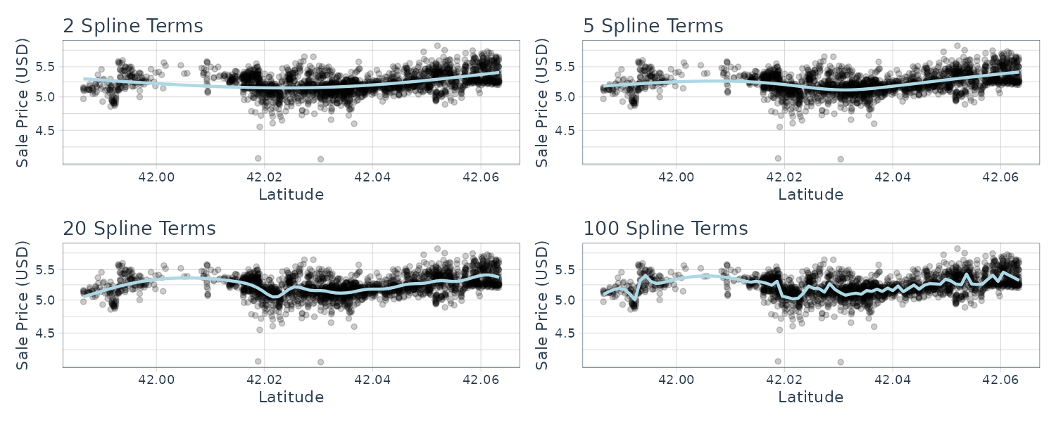
PCA
In the Ames data, several predictors measure size of the property such as total basement size (Total_Bsmt_SF), size of the first floor (First_Flr_SF), gross living area (Gr_Liv_Area), etc. We can use the following recipe step:
step_pca(matches("(SF$)|(Gr_Liv)")) This will convert the columns matching the regex and turn them into PC1, …, PC5 (default number of components to keep is 5).
Row Sampling
Downsampling the data keeps the minority class and takes a random sample of the majority class so class frequencies are balanced.
Upsampling replicates samples from the minority class.
step_upsample(outcome_column_name)
step_downsample(outcome_column_name)
General Transformations
step_mutate() can be used to conduct straightforward transformations:
step_mutate(
    Bedroom_Bath_Ratio = Bedroom_AbvGr / Full_Bath
  )
skip = TRUE
Certain step recipes should not be applied to the predict() function. For example downsampling should not be applied during predict() but applied when using fit(). By default, skip = TRUE for step_downsample().
Getting Info from tidy()
We can get a summary of the recipe steps via tidy():
> tidy(simple_ames)
# A tibble: 5 × 6
  number operation type     trained skip  id
   <int> <chr>     <chr>    <lgl>   <lgl> <chr>
1      1 step      log      FALSE   FALSE log_8fJH6
2      2 step      other    FALSE   FALSE other_1UZrP
3      3 step      dummy    FALSE   FALSE dummy_73XYf
4      4 step      interact FALSE   FALSE interact_RwEJr
5      5 step      pca      FALSE   FALSE pca_asXOF

estimated_recipe <- lm_fit |>
  extract_recipe(estimated = TRUE)
> tidy(estimated_recipe)
# A tibble: 5 × 6
  number operation type     trained skip  id
   <int> <chr>     <chr>    <lgl>   <lgl> <chr>
1      1 step      log      TRUE    FALSE log_8fJH6
2      2 step      other    TRUE    FALSE other_1UZrP
3      3 step      dummy    TRUE    FALSE dummy_73XYf
4      4 step      interact TRUE    FALSE interact_RwEJr
5      5 step      pca      TRUE    FALSE pca_asXOF
We can also get more info via the id parameter:
> tidy(estimated_recipe, id = "other_1UZrP")
# A tibble: 20 × 3
   terms        retained                                id
   <chr>        <chr>                                   <chr>
 1 Neighborhood North_Ames                              other_1UZrP
 2 Neighborhood College_Creek                           other_1UZrP
 3 Neighborhood Old_Town                                other_1UZrP
 4 Neighborhood Edwards                                 other_1UZrP
 5 Neighborhood Somerset                                other_1UZrP
 6 Neighborhood Northridge_Heights                      other_1UZrP
 7 Neighborhood Gilbert                                 other_1UZrP
 8 Neighborhood Sawyer                                  other_1UZrP
 9 Neighborhood Northwest_Ames                          other_1UZrP
10 Neighborhood Sawyer_West                             other_1UZrP
11 Neighborhood Mitchell                                other_1UZrP
12 Neighborhood Brookside                               other_1UZrP
13 Neighborhood Crawford                                other_1UZrP
14 Neighborhood Iowa_DOT_and_Rail_Road                  other_1UZrP
15 Neighborhood Timberland                              other_1UZrP
16 Neighborhood Northridge                              other_1UZrP
17 Neighborhood Stone_Brook                             other_1UZrP
18 Neighborhood South_and_West_of_Iowa_State_University other_1UZrP
19 Neighborhood Clear_Creek                             other_1UZrP
20 Neighborhood Meadow_Village                          other_1UZrP

> tidy(estimated_recipe, id = "pca_asXOF")
# A tibble: 25 × 4
   terms                              value component id
   <chr>                              <dbl> <chr>     <chr>
 1 Gr_Liv_Area                      -0.995  PC1       pca_asXOF
 2 Gr_Liv_Area_x_Bldg_Type_TwoFmCon -0.0194 PC1       pca_asXOF
 3 Gr_Liv_Area_x_Bldg_Type_Duplex   -0.0355 PC1       pca_asXOF
 4 Gr_Liv_Area_x_Bldg_Type_Twnhs    -0.0333 PC1       pca_asXOF
 5 Gr_Liv_Area_x_Bldg_Type_TwnhsE   -0.0842 PC1       pca_asXOF
 6 Gr_Liv_Area                       0.0786 PC2       pca_asXOF
 7 Gr_Liv_Area_x_Bldg_Type_TwoFmCon  0.0285 PC2       pca_asXOF
 8 Gr_Liv_Area_x_Bldg_Type_Duplex    0.0725 PC2       pca_asXOF
 9 Gr_Liv_Area_x_Bldg_Type_Twnhs     0.0646 PC2       pca_asXOF
10 Gr_Liv_Area_x_Bldg_Type_TwnhsE   -0.992  PC2       pca_asXOF
# ℹ 15 more rows
# ℹ Use `print(n = ...)` to see more rows
Column Roles
Suppose ames have a column of address that you want to leave in dataset but not use in modelling. This could be helpful when data are resampled and tracking which is which. This can be done with:
simple_ames |>
  update_role(address, new_role = "street address")
Metrics
Regression Metrics
Using the yardstick package, we can produce performance metrics. For example, taking the regression model we fitted earlier, we evaluate the performance on the test set:
ames_test_res <- predict(
  lm_fit,
  new_data = ames_test |>
    select(-Sale_Price)
) |>
  bind_cols(
    ames_test |> select(Sale_Price)
  )

> ames_test_res
# A tibble: 588 × 2
   .pred Sale_Price
   <dbl>      <dbl>
 1  5.22       5.02
 2  5.21       5.39
 3  5.28       5.28
 4  5.27       5.28
 5  5.28       5.28
 6  5.28       5.26
 7  5.26       5.73
 8  5.26       5.60
 9  5.26       5.32
10  5.24       4.98
# ℹ 578 more rows
# ℹ Use `print(n = ...)` to see more rows

> rmse(
  ames_test_res,
  truth = Sale_Price,
  estimate = .pred
)
# A tibble: 1 × 3
  .metric .estimator .estimate
  <chr>   <chr>          <dbl>
1 rmse    standard       0.168
To compute multiple metrics at once, we can use a metric set:
> metric_set(rmse, rsq, mae)(
  ames_test_res,
  truth = Sale_Price,
  estimate = .pred
)
# A tibble: 3 × 3
  .metric .estimator .estimate
  <chr>   <chr>          <dbl>
1 rmse    standard       0.168
2 rsq     standard       0.200
3 mae     standard       0.125
Binary Classification Metrics
We will use two_class_example dataset in modeldata package to demonstrate classification metrics:
tibble(two_class_example)
# A tibble: 500 × 4
   truth   Class1   Class2 predicted
   <fct>    <dbl>    <dbl> <fct>
 1 Class2 0.00359 0.996    Class2
 2 Class1 0.679   0.321    Class1
 3 Class2 0.111   0.889    Class2
 4 Class1 0.735   0.265    Class1
 5 Class2 0.0162  0.984    Class2
 6 Class1 0.999   0.000725 Class1
 7 Class1 0.999   0.000799 Class1
 8 Class1 0.812   0.188    Class1
 9 Class2 0.457   0.543    Class2
10 Class2 0.0976  0.902    Class2
# ℹ 490 more rows
# ℹ Use `print(n = ...)` to see more rows
A variety of yardstick metrics:
# Confusion Matrix
> conf_mat(
  two_class_example,
  truth = truth,
  estimate = predicted
)
          Truth
Prediction Class1 Class2
    Class1    227     50
    Class2     31    192

# Accuracy
> accuracy(
  two_class_example,
  truth = truth,
  estimate = predicted
)
# A tibble: 1 × 3
  .metric  .estimator .estimate
  <chr>    <chr>          <dbl>
1 accuracy binary         0.838

# Matthews Correlation Coefficient
> mcc(
  two_class_example,
  truth,
  predicted
)
# A tibble: 1 × 3
  .metric .estimator .estimate
  <chr>   <chr>          <dbl>
1 mcc     binary         0.677

# F1 Metric
> f_meas(
  two_class_example,
  truth,
  predicted
)
# A tibble: 1 × 3
  .metric .estimator .estimate
  <chr>   <chr>          <dbl>
1 f_meas  binary         0.849
Or combining all 3:
classification_metrics <- metric_set(
  accuracy,
  mcc,
  f_meas
)

> classification_metrics(
  two_class_example,
  truth = truth,
  estimate = predicted
)

# A tibble: 3 × 3
  .metric  .estimator .estimate
  <chr>    <chr>          <dbl>
1 accuracy binary         0.838
2 mcc      binary         0.677
3 f_meas   binary         0.849
The f_meas() metric emphasizes the positive class (event of interest). By default, the first level of the outcome factor is the event of interest. We can use the event_level argument to indicate which is the positive class:
f_meas(
  two_class_example,
  truth,
  predicted,
  event_level = "second"
)
There are other classification metrics that use the predicted probabilities as inputs rather than hard class predictions. For example, the Receiver Operating Characteristic (ROC) curve computes the sensitivy and specificity over a continuum of different event thresholds.
> roc_curve(
  two_class_example,
  truth,
  Class1
)
# A tibble: 502 × 3
   .threshold specificity sensitivity
        <dbl>       <dbl>       <dbl>
 1 -Inf           0                 1
 2    1.79e-7     0                 1
 3    4.50e-6     0.00413           1
 4    5.81e-6     0.00826           1
 5    5.92e-6     0.0124            1
 6    1.22e-5     0.0165            1
 7    1.40e-5     0.0207            1
 8    1.43e-5     0.0248            1
 9    2.38e-5     0.0289            1
10    3.30e-5     0.0331            1
# ℹ 492 more rows
# ℹ Use `print(n = ...)` to see more rows

> roc_auc(
  two_class_example,
  truth,
  Class1
)
# A tibble: 1 × 3
  .metric .estimator .estimate
  <chr>   <chr>          <dbl>
1 roc_auc binary         0.939
Plotting the ROC curve:
roc_curve(
  two_class_example,
  truth,
  Class1
) |>
  autoplot()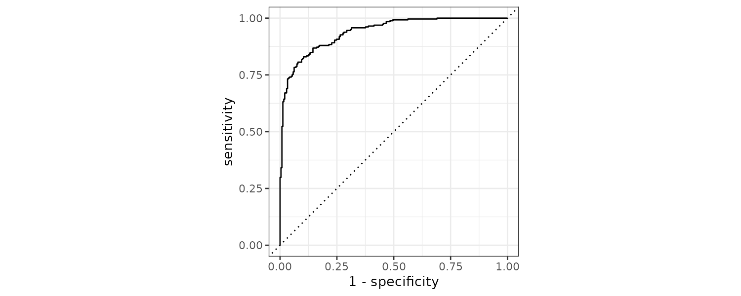
If the curve is close to the diagonal line, the model’s predictions would be no matter than random guessing.
Multiclass Classification Metrics
Using the hpc_cv dataset:
> tibble(hpc_cv)
# A tibble: 3,467 × 7
   obs   pred     VF      F       M          L Resample
   <fct> <fct> <dbl>  <dbl>   <dbl>      <dbl> <chr>
 1 VF    VF    0.914 0.0779 0.00848 0.0000199  Fold01
 2 VF    VF    0.938 0.0571 0.00482 0.0000101  Fold01
 3 VF    VF    0.947 0.0495 0.00316 0.00000500 Fold01
 4 VF    VF    0.929 0.0653 0.00579 0.0000156  Fold01
 5 VF    VF    0.942 0.0543 0.00381 0.00000729 Fold01
 6 VF    VF    0.951 0.0462 0.00272 0.00000384 Fold01
 7 VF    VF    0.914 0.0782 0.00767 0.0000354  Fold01
 8 VF    VF    0.918 0.0744 0.00726 0.0000157  Fold01
 9 VF    VF    0.843 0.128  0.0296  0.000192   Fold01
10 VF    VF    0.920 0.0728 0.00703 0.0000147  Fold01
# ℹ 3,457 more rows
# ℹ Use `print(n = ...)` to see more rows
The hpc dataset contains the predicted classes and class probabilities for a linear discriminant analysis model fit to the HPC data set from Kuhn and Johnson (2013). These data are the assessment sets from a 10-fold cross-validation scheme. The data column columns for the true class (‘obs’), the class prediction(‘pred’) and columns for each class probability (columns ‘VF’, ‘F’, ‘M’, and ‘L’). Additionally, a column for the resample indicator is included.
> conf_mat(
  hpc_cv,
  truth = obs,
  estimate = pred
)
          Truth
Prediction   VF    F    M    L
        VF 1620  371   64    9
        F   141  647  219   60
        M     6   24   79   28
        L     2   36   50  111

> accuracy(
  hpc_cv,
  obs,
  pred
)
# A tibble: 1 × 3
  .metric  .estimator .estimate
  <chr>    <chr>          <dbl>
1 accuracy multiclass     0.709

> mcc(
  hpc_cv,
  obs,
  pred
)
# A tibble: 1 × 3
  .metric .estimator .estimate
  <chr>   <chr>          <dbl>
1 mcc     multiclass     0.515
Note that the estimator is “multiclass” vs the previous “binary”.
Sensitivity
There are a few ways to calculate sensitivity to multiclass classification. Below we set up some code that can be used to calculate sensitivity:
class_totals <- count(
  hpc_cv,
  obs,
  name = "totals"
) |>
  mutate(class_wts = totals / sum(totals))
> class_totals
  obs totals  class_wts
1  VF   1769 0.51023940
2   F   1078 0.31093164
3   M    412 0.11883473
4   L    208 0.05999423

cell_counts <- hpc_cv |>
  group_by(obs, pred) |>
  count() |>
  ungroup()
> cell_counts
# A tibble: 16 × 3
   obs   pred      n
   <fct> <fct> <int>
 1 VF    VF     1620
 2 VF    F       141
 3 VF    M         6
 4 VF    L         2
 5 F     VF      371
 6 F     F       647
 7 F     M        24
 8 F     L        36
 9 M     VF       64
10 M     F       219
11 M     M        79
12 M     L        50
13 L     VF        9
14 L     F        60
15 L     M        28
16 L     L       111

one_versus_all <- cell_counts |>
  filter(obs == pred) |>
  full_join(class_totals, by = "obs") |>
  mutate(sens = n / totals)

> one_versus_all
# A tibble: 4 × 6
  obs   pred      n totals class_wts  sens
  <fct> <fct> <int>  <int>     <dbl> <dbl>
1 VF    VF     1620   1769    0.510  0.916
2 F     F       647   1078    0.311  0.600
3 M     M        79    412    0.119  0.192
4 L     L       111    208    0.0600 0.534
Macro-Averaging
Computes a set of on-versus-all metrics and averaging it:
> one_versus_all |>
  summarize(
    macro = mean(sens)
  )
# A tibble: 1 × 1
  macro
  <dbl>
1 0.560

> sensitivity(
  hpc_cv,
  obs,
  pred,
  estimator = "macro"
)
# A tibble: 1 × 3
  .metric     .estimator .estimate
  <chr>       <chr>          <dbl>
1 sensitivity macro          0.560
Macro-Weighted Averaging
The average is weighted by the number of samples in each class:
> one_versus_all |>
  summarize(
    macro_wts = weighted.mean(sens, class_wts)
  )
# A tibble: 1 × 1
  macro_wts
  <dbl>
1 0.709

> sensitivity(
  hpc_cv,
  obs,
  pred,
  estimator = "macro_weighted"
)
# A tibble: 1 × 3
  .metric     .estimator     .estimate
  <chr>       <chr>              <dbl>
1 sensitivity macro_weighted     0.709
Micro-Averaging
Aggregating the totals for each class, and then computes a single metric from the aggregates:
> one_versus_all |>
  summarize(
    micro = sum(n) / sum(totals)
  )
# A tibble: 1 × 1
  macro_wts
  <dbl>
1 0.709

> sensitivity(
  hpc_cv,
  obs,
  pred,
  estimator = "micro"
)
# A tibble: 1 × 3
  .metric     .estimator .estimate
  <chr>       <chr>          <dbl>
1 sensitivity micro          0.709
Multiclass ROC:
There are multiclass analog for ROC as well:
> roc_auc(hpc_cv, obs, VF, F, M, L)
# A tibble: 1 × 3
  .metric .estimator .estimate
  <chr>   <chr>          <dbl>
1 roc_auc hand_till      0.829

roc_curve(hpc_cv, obs, VF, F, M, L) |>
  autoplot()
We can plot the ROC curve for each group by the folds:
hpc_cv |>
  group_by(Resample) |>
  roc_curve(obs, VF, F, M, L) |>
  autoplot() +
theme(legend.position = "none") 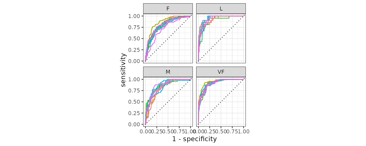
Grouping the accuracy by resampling groups:
> hpc_cv |>
  group_by(Resample) |>
  accuracy(obs, pred)
# A tibble: 10 × 4
   Resample .metric  .estimator .estimate
   <chr>    <chr>    <chr>          <dbl>
 1 Fold01   accuracy multiclass     0.726
 2 Fold02   accuracy multiclass     0.712
 3 Fold03   accuracy multiclass     0.758
 4 Fold04   accuracy multiclass     0.712
 5 Fold05   accuracy multiclass     0.712
 6 Fold06   accuracy multiclass     0.697
 7 Fold07   accuracy multiclass     0.675
 8 Fold08   accuracy multiclass     0.721
 9 Fold09   accuracy multiclass     0.673
10 Fold10   accuracy multiclass     0.699
Resampling
When we measure performance on the same data that we used for training, the data is said to be resubstituted.
Predictive models that are capable of learning complex trends are known as low bias models. Many black-box ML models have low bias, while models such as linear regression and discriminant analysis are less adaptable and are considered high bias models.
Resampling is only conducted on the training set. For each iteration of resampling, the data are partitioned into an analysis set and an assessment set. Model is fit on the analysis set and evaluated on the assessment set.
Cross-Validation
Generally we prefer a 10-fold cross-validation as a default. Larger values result in resampling estimates with small bias but large variance, while smaller values have large bias but low variance.
ames_folds <- vfold_cv(ames_train, v = 10)
> ames_folds
#  10-fold cross-validation
# A tibble: 10 × 2
   splits             id
   <list>             <chr>
 1 <split [2107/235]> Fold01
 2 <split [2107/235]> Fold02
 3 <split [2108/234]> Fold03
 4 <split [2108/234]> Fold04
 5 <split [2108/234]> Fold05
 6 <split [2108/234]> Fold06
 7 <split [2108/234]> Fold07
 8 <split [2108/234]> Fold08
 9 <split [2108/234]> Fold09
10 <split [2108/234]> Fold10
The column splits contains the information on how to split the data (training/test). Note that data is not replicated in memory for the folds. We can show this by noticing the object size of ames_folds are not 10 times the size of ames_train:
> lobstr::obj_size(ames_train)
849.83 kB

> lobstr::obj_size(ames_folds)
944.36 kB
To retrieve the first fold training data:
> ames_folds$splits[[1]] |>
  analysis() |>
  select(1:5)
# A tibble: 2,107 × 5
   MS_SubClass                         MS_Zoning                  Lot_Frontage Lot_Area Street
   <fct>                               <fct>                             <dbl>    <int> <fct>
 1 One_Story_1946_and_Newer_All_Styles Residential_Low_Density              70     8400 Pave
 2 One_Story_1946_and_Newer_All_Styles Residential_Low_Density              70    10500 Pave
 3 Two_Story_PUD_1946_and_Newer        Residential_Medium_Density           21     1680 Pave
 4 Two_Story_PUD_1946_and_Newer        Residential_Medium_Density           21     1680 Pave
 5 One_Story_PUD_1946_and_Newer        Residential_Low_Density              53     4043 Pave
 6 One_Story_PUD_1946_and_Newer        Residential_Low_Density              24     2280 Pave
 7 One_Story_PUD_1946_and_Newer        Residential_Low_Density              55     7892 Pave
 8 One_Story_1945_and_Older            Residential_High_Density             70     9800 Pave
 9 Duplex_All_Styles_and_Ages          Residential_Medium_Density           68     8930 Pave
10 One_Story_1946_and_Newer_All_Styles Residential_Low_Density               0     9819 Pave
# ℹ 2,097 more rows
# ℹ Use `print(n = ...)` to see more rows
And test set:
> ames_folds$splits[[1]] |>
  assessment() |>
  select(1:5)
# A tibble: 235 × 5
   MS_SubClass                               MS_Zoning                  Lot_Frontage Lot_Area Street
   <fct>                                     <fct>                             <dbl>    <int> <fct>
 1 One_and_Half_Story_Finished_All_Ages      Residential_Low_Density              60     8382 Pave
 2 One_Story_1945_and_Older                  Residential_Medium_Density           60     7200 Pave
 3 One_and_Half_Story_Finished_All_Ages      Residential_Medium_Density            0     8239 Pave
 4 Two_Family_conversion_All_Styles_and_Ages Residential_Medium_Density          100     9045 Pave
 5 One_Story_1946_and_Newer_All_Styles       Residential_Low_Density               0    11200 Pave
 6 One_and_Half_Story_Finished_All_Ages      C_all                                66     8712 Pave
 7 One_Story_1946_and_Newer_All_Styles       Residential_Low_Density              70     9100 Pave
 8 One_Story_1946_and_Newer_All_Styles       Residential_Low_Density             120    13560 Pave
 9 One_Story_1946_and_Newer_All_Styles       Residential_Low_Density              60    10434 Pave
10 One_Story_1946_and_Newer_All_Styles       Residential_Low_Density              75     9533 Pave
# ℹ 225 more rows
# ℹ Use `print(n = ...)` to see more rows
Repeated CV
Depending on the size of the data, the V-fold CV can be noisy. One way to reduce the noise is to repeat V-fold multiple times (R times). The standard error would then be \(\frac{\sigma}{\sqrt{V\times R}}\).
As long as we have a lot of data relative to VxR, the summary statistics will tend toward a normal distribution by CLT.
> vfold_cv(ames_train, v = 10, repeats = 5)
#  10-fold cross-validation repeated 5 times
# A tibble: 50 × 3
   splits             id      id2
   <list>             <chr>   <chr>
 1 <split [2107/235]> Repeat1 Fold01
 2 <split [2107/235]> Repeat1 Fold02
 3 <split [2108/234]> Repeat1 Fold03
 4 <split [2108/234]> Repeat1 Fold04
 5 <split [2108/234]> Repeat1 Fold05
 6 <split [2108/234]> Repeat1 Fold06
 7 <split [2108/234]> Repeat1 Fold07
 8 <split [2108/234]> Repeat1 Fold08
 9 <split [2108/234]> Repeat1 Fold09
10 <split [2108/234]> Repeat1 Fold10
# ℹ 40 more rows
# ℹ Use `print(n = ...)` to see more rows
Monte Carlo Cross-Validation (MCCV)
The difference between MCCV and CV is that the data in each fold is randomly selected:
> mc_cv(
  ames_train,
  prop = 9 / 10,
  times = 20
)
# Monte Carlo cross-validation (0.9/0.1) with 20 resamples
# A tibble: 20 × 2
   splits             id
   <list>             <chr>
 1 <split [2107/235]> Resample01
 2 <split [2107/235]> Resample02
 3 <split [2107/235]> Resample03
 4 <split [2107/235]> Resample04
 5 <split [2107/235]> Resample05
 6 <split [2107/235]> Resample06
 7 <split [2107/235]> Resample07
 8 <split [2107/235]> Resample08
 9 <split [2107/235]> Resample09
10 <split [2107/235]> Resample10
11 <split [2107/235]> Resample11
12 <split [2107/235]> Resample12
13 <split [2107/235]> Resample13
14 <split [2107/235]> Resample14
15 <split [2107/235]> Resample15
16 <split [2107/235]> Resample16
17 <split [2107/235]> Resample17
18 <split [2107/235]> Resample18
19 <split [2107/235]> Resample19
20 <split [2107/235]> Resample20
This results in assessment sets that are not mutually exclusive.
Validation Sets
If the dataset is very large, it might be adequate to reserve a validation set and only do the validation once rather than CV.
val_set <- validation_split(
  ames_train,
  prop = 3 / 4
)

> val_set
# Validation Set Split (0.75/0.25)
# A tibble: 1 × 2
  splits             id
  <list>             <chr>
1 <split [1756/586]> validation
Bootstrapping
A bootstrap sample is a sample that is drawn with replacement. This mean that some data points might be selected more than once. Furthermore, each data point has a 63.2% chance of inclusion in the training set at least once. The assessment set contains all of the training set samples that were not selected for the analysis set. The assessment set is often called the out-of-bag sample.
> bootstraps(ames_train, times = 5)
# Bootstrap sampling
# A tibble: 5 × 2
  splits             id
  <list>             <chr>
1 <split [2342/854]> Bootstrap1
2 <split [2342/846]> Bootstrap2
3 <split [2342/857]> Bootstrap3
4 <split [2342/861]> Bootstrap4
5 <split [2342/871]> Bootstrap5
Compared to CV, bootstrapping has low variance but high bias. For example, if the true accuracy of the model is 90%, bootstrapping will tend to estimate value less than 90%.
Rolling Forecasts
Time series forecast require a rolling resampling. In this example, a training set of 6 samples is sampled with an assessment (validation) size of 30 days, with a 29 day skip:
time_slices <- tibble(x = 1:365) |>
  rolling_origin(
    initial = 6 * 30,
    assess = 30,
    skip = 29,
    cumulative = FALSE
  )

> time_slices
# Rolling origin forecast resampling
# A tibble: 6 × 2
  splits           id
  <list>           <chr>
1 <split [180/30]> Slice1
2 <split [180/30]> Slice2
3 <split [180/30]> Slice3
4 <split [180/30]> Slice4
5 <split [180/30]> Slice5
6 <split [180/30]> Slice6
The analysis() function shows the indices of training set and assessment() function shows the indices of validation set:
data_range <- function(x) {
  summarize(
    x,
    first = min(x),
    last = max(x)
  )
}

> map_dfr(
  time_slices$splits,
  ~ analysis(.x) |>
    data_range()
)
# A tibble: 6 × 2
  first  last
  <int> <int>
1     1   180
2    31   210
3    61   240
4    91   270
5   121   300
6   151   330

> map_dfr(
  time_slices$splits,
  ~ assessment(.x) |>
    data_range()
)
# A tibble: 6 × 2
  first  last
  <int> <int>
1   181   210
2   211   240
3   241   270
4   271   300
5   301   330
6   331   360
Estimating Performance
Using the earlier CV folds, we can run a resampling:
lm_res <- lm_wflow |>
  fit_resamples(
    resamples = ames_folds,
    control = control_resamples(
      save_pred = TRUE,
      save_workflow = TRUE
    )
  )

> lm_res
# Resampling results
# 10-fold cross-validation
# A tibble: 10 × 5
   splits             id     .metrics         .notes           .predictions
   <list>             <chr>  <list>           <list>           <list>
 1 <split [2107/235]> Fold01 <tibble [2 × 4]> <tibble [0 × 3]> <tibble [235 × 4]>
 2 <split [2107/235]> Fold02 <tibble [2 × 4]> <tibble [0 × 3]> <tibble [235 × 4]>
 3 <split [2108/234]> Fold03 <tibble [2 × 4]> <tibble [0 × 3]> <tibble [234 × 4]>
 4 <split [2108/234]> Fold04 <tibble [2 × 4]> <tibble [0 × 3]> <tibble [234 × 4]>
 5 <split [2108/234]> Fold05 <tibble [2 × 4]> <tibble [0 × 3]> <tibble [234 × 4]>
 6 <split [2108/234]> Fold06 <tibble [2 × 4]> <tibble [0 × 3]> <tibble [234 × 4]>
 7 <split [2108/234]> Fold07 <tibble [2 × 4]> <tibble [0 × 3]> <tibble [234 × 4]>
 8 <split [2108/234]> Fold08 <tibble [2 × 4]> <tibble [0 × 3]> <tibble [234 × 4]>
 9 <split [2108/234]> Fold09 <tibble [2 × 4]> <tibble [0 × 3]> <tibble [234 × 4]>
10 <split [2108/234]> Fold10 <tibble [2 × 4]> <tibble [0 × 3]> <tibble [234 × 4]>
.metrics contains the assessment set performance statistics.
.notes contains any warnings or errors generated during resampling.
.predictions contain out-of-sample predictions when save_pred = TRUE.
To obtain the performance metrics:
> collect_metrics(lm_res)
# A tibble: 2 × 6
  .metric .estimator  mean     n std_err .config
  <chr>   <chr>      <dbl> <int>   <dbl> <chr>
1 rmse    standard   0.160    10 0.00284 Preprocessor1_Model1
2 rsq     standard   0.178    10 0.0198  Preprocessor1_Model1
To obtain the assessment set predictions:
assess_res <- collect_predictions(lm_res)
> assess_res
# A tibble: 2,342 × 5
   id     .pred  .row Sale_Price .config
   <chr>  <dbl> <int>      <dbl> <chr>
 1 Fold01  5.29     9       5.09 Preprocessor1_Model1
 2 Fold01  5.28    48       5.10 Preprocessor1_Model1
 3 Fold01  5.25    50       5.09 Preprocessor1_Model1
 4 Fold01  5.26    58       5    Preprocessor1_Model1
 5 Fold01  5.25    78       5.11 Preprocessor1_Model1
 6 Fold01  5.24    80       5.08 Preprocessor1_Model1
 7 Fold01  5.23    90       5    Preprocessor1_Model1
 8 Fold01  5.32    91       5.08 Preprocessor1_Model1
 9 Fold01  5.19   106       5.04 Preprocessor1_Model1
10 Fold01  5.16   117       5.04 Preprocessor1_Model1
# ℹ 2,332 more rows
# ℹ Use `print(n = ...)` to see more rows
We can check for predictions that are way off by first plotting the prediction vs actual test set:
assess_res |>
  ggplot(aes(x = Sale_Price, y = .pred)) +
  geom_point(alpha = .15) +
  geom_abline(color = "red") +
  coord_obs_pred() +
  ylab("Predicted")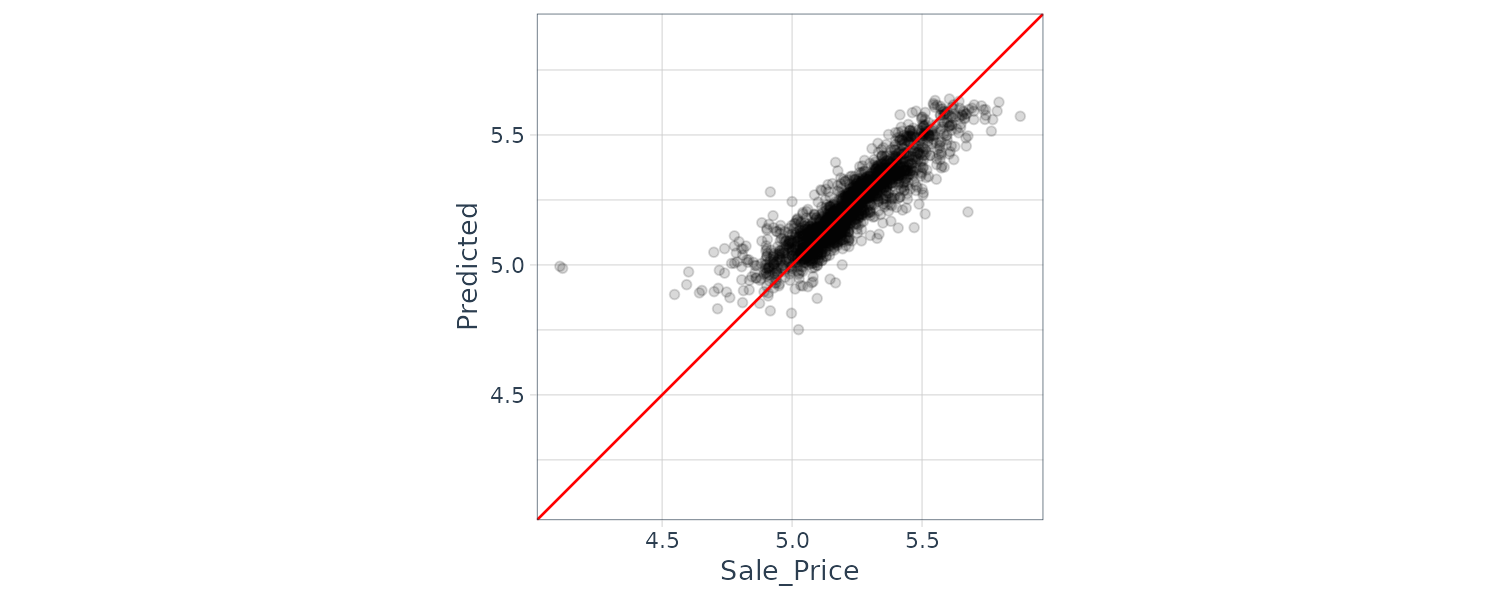
There are two houses in the test set that are overpredicted by the model:
over_predicted <- assess_res |>
  mutate(residual = Sale_Price - .pred) |>
  arrange(desc(abs(residual))) |>
  slice(1:2)

> over_predicted
# A tibble: 2 × 6
  id     .pred  .row Sale_Price .config
  <chr>  <dbl> <int>      <dbl> <chr>
1 Fold05  4.98   329       4.12 Prepro…
2 Fold03  4.95    26       4.11 Prepro…
# ℹ 1 more variable: residual <dbl>
We then search for the data rows in the training set:
> ames_train |>
  slice(over_predicted$.row) |>
  select(
    Gr_Liv_Area,
    Neighborhood,
    Year_Built,
    Bedroom_AbvGr,
    Full_Bath
  )
# A tibble: 2 × 5
  Gr_Liv_Area Neighborhood   Year_Built
        <int> <fct>               <int>
1         733 Iowa_DOT_and_…       1952
2         832 Old_Town             1923
# ℹ 2 more variables:
#   Bedroom_AbvGr <int>,
#   Full_Bath <int>
To use a validation set:
val_res <- lm_wflow |>
  fit_resamples(
    resamples = val_set
  )

> val_res
# Resampling results
# Validation Set Split (0.75/0.25)
# A tibble: 1 × 4
  splits             id        .metrics
  <list>             <chr>     <list>
1 <split [1756/586]> validati… <tibble>
# ℹ 1 more variable: .notes <list>

> collect_metrics(val_res)
# A tibble: 2 × 6
  .metric .estimator   mean     n
  <chr>   <chr>       <dbl> <int>
1 rmse    standard   0.0820     1
2 rsq     standard   0.790      1
# ℹ 2 more variables: std_err <dbl>,
#   .config <chr>
Parallel Processing
The number of possible worker possible worker processes is determined by the parallel package:
# number of physical cores
> parallel::detectCores(logical = FALSE)
[1] 6

# number of independent simultaneous processes that can be used
> parallel::detectCores(logical = TRUE)
[1] 6
For fit_resamples() and other functions in tune, the user need to register a parallel backend package. On Unix we can load the doMC package:
# Unix only
library(doMC)
registerDoMC(cores = 2)
# Now run fit_resamples()...

# To reset the computations to sequential processing
registerDoSEQ()
For all operating systems, we can use the doParallel package:
library(doParallel)
# Create a cluster object and then register:
cl <- makePSOCKcluster(2)
registerDoParallel(cl)
# Now run fit_resamples()`...
stopCluster(cl)
Depending on the data and model type, the linear speed-up deteriorates after four to five cores. Note also that memory use will be increased as the data set is replicated across multiple core processes.
Saving the Resampled Objects
The models created during resampling are not retained. However, we can extract information of the models.
Let us review what we currently have for recipe:
ames_rec <- recipe(
  Sale_Price ~ Neighborhood +
    Gr_Liv_Area +
    Year_Built +
    Bldg_Type +
    Latitude +
    Longitude,
  data = ames_train
) |>
step_other(Neighborhood, threshold = 0.01) |>
step_dummy(all_nominal_predictors()) |>
step_interact( ~ Gr_Liv_Area:starts_with("Bldg_Type_") ) |>
step_ns(Latitude, Longitude, deg_free = 20)

lm_wflow <- workflow() |>
  add_recipe(ames_rec) |>
  add_model(
    linear_reg() |>
      set_engine("lm")
  )

lm_fit <- lm_wflow |>
  fit(data = ames_train)

> extract_recipe(
  lm_fit,
  estimated = TRUE
)
── Recipe ───────────────────────────────────────────────────────────────

── Inputs
Number of variables by role
outcome:   1
predictor: 6

── Training information
Training data contained 2342 data points and no incomplete rows.

── Operations
• Collapsing factor levels for: Neighborhood | Trained
• Dummy variables from: Neighborhood, Bldg_Type | Trained
• Interactions with: Gr_Liv_Area:(Bldg_Type_TwoFmCon + Bldg_Type_Duplex +
  Bldg_Type_Twnhs + Bldg_Type_TwnhsE) | Trained
• Natural splines on: Latitude, Longitude | Trained
To save and extract the linear model coefficients from a workflow:
ames_folds <- vfold_cv(ames_train, v = 10)

lm_res <- lm_wflow |>
  fit_resamples(
    resamples = ames_folds,
    control = control_resamples(
      extract = function(x) {
        extract_fit_parsnip(x) |>
          tidy()
      }
    )
  )

> lm_res
# Resampling results
# 10-fold cross-validation
# A tibble: 10 × 5
   splits             id     .metrics         .notes           .extracts
   <list>             <chr>  <list>           <list>           <list>
 1 <split [2107/235]> Fold01 <tibble [2 × 4]> <tibble [0 × 3]> <tibble [1 × 2]>
 2 <split [2107/235]> Fold02 <tibble [2 × 4]> <tibble [0 × 3]> <tibble [1 × 2]>
 3 <split [2108/234]> Fold03 <tibble [2 × 4]> <tibble [0 × 3]> <tibble [1 × 2]>
 4 <split [2108/234]> Fold04 <tibble [2 × 4]> <tibble [0 × 3]> <tibble [1 × 2]>
 5 <split [2108/234]> Fold05 <tibble [2 × 4]> <tibble [0 × 3]> <tibble [1 × 2]>
 6 <split [2108/234]> Fold06 <tibble [2 × 4]> <tibble [0 × 3]> <tibble [1 × 2]>
 7 <split [2108/234]> Fold07 <tibble [2 × 4]> <tibble [0 × 3]> <tibble [1 × 2]>
 8 <split [2108/234]> Fold08 <tibble [2 × 4]> <tibble [0 × 3]> <tibble [1 × 2]>
 9 <split [2108/234]> Fold09 <tibble [2 × 4]> <tibble [0 × 3]> <tibble [1 × 2]>
10 <split [2108/234]> Fold10 <tibble [2 × 4]> <tibble [0 × 3]> <tibble [1 × 2]>
An example to extract 2 folds coefficients:
> lm_res$.extracts[[1]][[1]]
[[1]]
# A tibble: 71 × 5
   term                             estimate  std.error statistic   p.value
   <chr>                               <dbl>      <dbl>     <dbl>     <dbl>
 1 (Intercept)                      1.08     0.329          3.28  1.05e-  3
 2 Gr_Liv_Area                      0.000176 0.00000485    36.3   5.01e-223
 3 Year_Built                       0.00210  0.000152      13.8   2.75e- 41
 4 Neighborhood_College_Creek      -0.0628   0.0366        -1.71  8.65e-  2
 5 Neighborhood_Old_Town           -0.0572   0.0139        -4.12  4.02e-  5
 6 Neighborhood_Edwards            -0.129    0.0303        -4.25  2.28e-  5
 7 Neighborhood_Somerset            0.0582   0.0209         2.79  5.37e-  3
 8 Neighborhood_Northridge_Heights  0.0845   0.0309         2.74  6.24e-  3
 9 Neighborhood_Gilbert            -0.00883  0.0249        -0.355 7.23e-  1
10 Neighborhood_Sawyer             -0.130    0.0289        -4.50  7.29e-  6
# ℹ 61 more rows
# ℹ Use `print(n = ...)` to see more rows

> lm_res$.extracts[[10]][[1]]
[[1]]
# A tibble: 71 × 5
   term                             estimate  std.error statistic   p.value
   <chr>                               <dbl>      <dbl>     <dbl>     <dbl>
 1 (Intercept)                      1.17     0.330          3.56  3.82e-  4
 2 Gr_Liv_Area                      0.000173 0.00000469    36.9   2.37e-228
 3 Year_Built                       0.00198  0.000154      12.8   2.99e- 36
 4 Neighborhood_College_Creek       0.0127   0.0369         0.345 7.30e-  1
 5 Neighborhood_Old_Town           -0.0467   0.0139        -3.35  8.21e-  4
 6 Neighborhood_Edwards            -0.109    0.0294        -3.70  2.18e-  4
 7 Neighborhood_Somerset            0.0358   0.0209         1.71  8.70e-  2
 8 Neighborhood_Northridge_Heights  0.0636   0.0313         2.04  4.18e-  2
 9 Neighborhood_Gilbert            -0.0165   0.0252        -0.656 5.12e-  1
10 Neighborhood_Sawyer             -0.118    0.0282        -4.18  3.06e-  5
# ℹ 61 more rows
# ℹ Use `print(n = ...)` to see more rows
All the results can be flattened into a tibble:
all_coef <- map_dfr(
  lm_res$.extracts,
  ~ .x[[1]][[1]]
)

> all_coef
# A tibble: 718 × 5
   term                             estimate  std.error statistic   p.value
   <chr>                               <dbl>      <dbl>     <dbl>     <dbl>
 1 (Intercept)                      1.12     0.313          3.58  3.48e-  4
 2 Gr_Liv_Area                      0.000166 0.00000469    35.3   1.87e-213
 3 Year_Built                       0.00202  0.000148      13.6   1.19e- 40
 4 Neighborhood_College_Creek      -0.0795   0.0365        -2.18  2.96e-  2
 5 Neighborhood_Old_Town           -0.0642   0.0132        -4.87  1.18e-  6
 6 Neighborhood_Edwards            -0.151    0.0290        -5.20  2.25e-  7
 7 Neighborhood_Somerset            0.0554   0.0202         2.75  6.03e-  3
 8 Neighborhood_Northridge_Heights  0.0948   0.0286         3.32  9.32e-  4
 9 Neighborhood_Gilbert            -0.00743  0.0225        -0.331 7.41e-  1
10 Neighborhood_Sawyer             -0.163    0.0276        -5.91  4.12e-  9
# ℹ 708 more rows
# ℹ Use `print(n = ...)` to see more rows

> filter(all_coef, term == "Year_Built")
# A tibble: 10 × 5
   term       estimate std.error statistic  p.value
   <chr>         <dbl>     <dbl>     <dbl>    <dbl>
 1 Year_Built  0.00202  0.000148      13.6 1.19e-40
 2 Year_Built  0.00192  0.000146      13.1 7.02e-38
 3 Year_Built  0.00193  0.000145      13.3 6.73e-39
 4 Year_Built  0.00200  0.000142      14.1 5.68e-43
 5 Year_Built  0.00201  0.000142      14.2 1.68e-43
 6 Year_Built  0.00188  0.000142      13.2 2.88e-38
 7 Year_Built  0.00193  0.000143      13.5 6.99e-40
 8 Year_Built  0.00201  0.000144      13.9 2.69e-42
 9 Year_Built  0.00192  0.000141      13.7 7.41e-41
10 Year_Built  0.00190  0.000144      13.2 1.79e-38
Comparing Models
Let us create 3 different linear models that add interaction and spline incrementally:
basic_rec <- recipe(
  Sale_Price ~ Neighborhood +
    Gr_Liv_Area +
    Year_Built +
    Bldg_Type +
    Latitude +
    Longitude,
  data = ames_train) |>
  step_log(Gr_Liv_Area, base = 10) |>
  step_other(Neighborhood, threshold = 0.01) |>
  step_dummy(all_nominal_predictors())

interaction_rec <- basic_rec |>
  step_interact(~ Gr_Liv_Area:starts_with("Bldg_Type_"))

spline_rec <- interaction_rec |>
  step_ns(Latitude, Longitude, deg_free = 50)

preproc <- list(
    basic = basic_rec,
    interact = interaction_rec,
    splines = spline_rec
  )

lm_models <- workflow_set(
  preproc,
  list(lm = linear_reg()),
  cross = FALSE
)

> lm_models
# A workflow set/tibble: 3 × 4
  wflow_id    info             option    result
  <chr>       <list>           <list>    <list>
1 basic_lm    <tibble [1 × 4]> <opts[0]> <list [0]>
2 interact_lm <tibble [1 × 4]> <opts[0]> <list [0]>
3 splines_lm  <tibble [1 × 4]> <opts[0]> <list [0]>
Using workflow_map(), we will run resampling for each model:
lm_models <- lm_models |>
  workflow_map(
    "fit_resamples",
    seed = 1101,
    verbose = TRUE,
    resamples = ames_folds,
    control = control_resamples(
      save_pred = TRUE,
      save_workflow = TRUE
    )
  )

> lm_models
# A workflow set/tibble: 3 × 4
  wflow_id    info             option    result
  <chr>       <list>           <list>    <list>
1 basic_lm    <tibble [1 × 4]> <opts[2]> <rsmp[+]>
2 interact_lm <tibble [1 × 4]> <opts[2]> <rsmp[+]>
3 splines_lm  <tibble [1 × 4]> <opts[2]> <rsmp[+]>
Using helper functions to report performance statistics:
> collect_metrics(lm_models) |>
  filter(.metric == "rmse")
# A tibble: 3 × 9
  wflow_id    .config              preproc model      .metric .estimator   mean     n std_err
  <chr>       <chr>                <chr>   <chr>      <chr>   <chr>       <dbl> <int>   <dbl>
1 basic_lm    Preprocessor1_Model1 recipe  linear_reg rmse    standard   0.0802    10 0.00231
2 interact_lm Preprocessor1_Model1 recipe  linear_reg rmse    standard   0.0797    10 0.00226
3 splines_lm  Preprocessor1_Model1 recipe  linear_reg rmse    standard   0.0792    10 0.00223
Now let’s add another random forest model to the workflow set:
rf_wflow <- workflow() |>
  add_recipe(ames_rec) |>
  add_model(
    rand_forest(trees = 1000, min_n = 5) |>
      set_engine("ranger") |>
      set_mode("regression")
  )

rf_res <- rf_wflow |>
  fit_resamples(
    resamples = ames_folds,
    control = control_resamples(
      save_pred = TRUE,
      save_workflow = TRUE
    )
  )

four_models <- as_workflow_set(
  random_forest = rf_res
) |>
  bind_rows(lm_models)

> four_models
# A workflow set/tibble: 4 × 4
  wflow_id      info             option    result
  <chr>         <list>           <list>    <list>
1 random_forest <tibble [1 × 4]> <opts[0]> <rsmp[+]>
2 basic_lm      <tibble [1 × 4]> <opts[2]> <rsmp[+]>
3 interact_lm   <tibble [1 × 4]> <opts[2]> <rsmp[+]>
4 splines_lm    <tibble [1 × 4]> <opts[2]> <rsmp[+]>
To plot the \(R^{2}\) confidence intervals for easy comparison:
library(ggrepel)
autoplot(four_models, metric = "rsq") +
  geom_text_repel(aes(label = wflow_id)) +
  theme(legend.position = "none")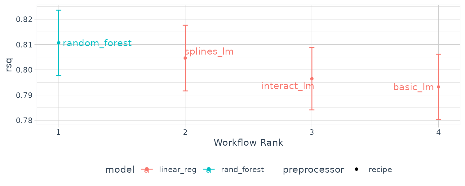
Let us gather and summarize the correlation of the resamnpling statistics across each models:
rsq_indiv_estimates <- collect_metrics(
  four_models,
  summarize = FALSE
) |>
  filter(.metric == "rsq")

> rsq_indiv_estimates
# A tibble: 40 × 8
   wflow_id      .config              preproc model       id     .metric .estimator .estimate
   <chr>         <chr>                <chr>   <chr>       <chr>  <chr>   <chr>          <dbl>
 1 random_forest Preprocessor1_Model1 recipe  rand_forest Fold01 rsq     standard       0.826
 2 random_forest Preprocessor1_Model1 recipe  rand_forest Fold02 rsq     standard       0.808
 3 random_forest Preprocessor1_Model1 recipe  rand_forest Fold03 rsq     standard       0.812
 4 random_forest Preprocessor1_Model1 recipe  rand_forest Fold04 rsq     standard       0.855
 5 random_forest Preprocessor1_Model1 recipe  rand_forest Fold05 rsq     standard       0.853
 6 random_forest Preprocessor1_Model1 recipe  rand_forest Fold06 rsq     standard       0.853
 7 random_forest Preprocessor1_Model1 recipe  rand_forest Fold07 rsq     standard       0.696
 8 random_forest Preprocessor1_Model1 recipe  rand_forest Fold08 rsq     standard       0.855
 9 random_forest Preprocessor1_Model1 recipe  rand_forest Fold09 rsq     standard       0.805
10 random_forest Preprocessor1_Model1 recipe  rand_forest Fold10 rsq     standard       0.841
# ℹ 30 more rows
# ℹ Use `print(n = ...)` to see more rows
rsq_wider <- rsq_indiv_estimates |>
select(wflow_id, .estimate, id) |>
pivot_wider(
id_cols = "id",
names_from = "wflow_id",
values_from = ".estimate"
)
> rsq_wider
# A tibble: 10 × 5
id random_forest basic_lm interact_lm splines_lm
<chr> <dbl> <dbl> <dbl> <dbl>
1 Fold01 0.807 0.781 0.791 0.808
2 Fold02 0.840 0.815 0.816 0.821
3 Fold03 0.835 0.804 0.811 0.820
4 Fold04 0.769 0.743 0.750 0.757
5 Fold05 0.828 0.794 0.789 0.783
6 Fold06 0.799 0.801 0.802 0.820
7 Fold07 0.842 0.821 0.822 0.831
8 Fold08 0.808 0.762 0.765 0.775
9 Fold09 0.790 0.794 0.798 0.804
10 Fold10 0.789 0.816 0.820 0.828
> corrr::correlate(
rsq_wider |>
select(-id),
quiet = TRUE
)
# A tibble: 4 × 5
term random_forest basic_lm interact_lm splines_lm
<chr> <dbl> <dbl> <dbl> <dbl>
1 random_forest NA 0.618 0.574 0.480
2 basic_lm 0.618 NA 0.987 0.922
3 interact_lm 0.574 0.987 NA 0.963
4 splines_lm 0.480 0.922 0.963 NAThere are large correlations across models implying a large within-resample correlations. Another way to view this is to plot each model with lines connecting the resamples:
rsq_indiv_estimates |>
  mutate(
    wflow_id = reorder(
      wflow_id,
      .estimate
    )
  ) |>
  ggplot(
    aes(
      x = wflow_id,
      y = .estimate,
      group = id,
      color = id,
      lty = id
    )
  ) +
  geom_line(
    alpha = .8,
    lwd = 1.25
  ) +
  theme(legend.position = "none") +
  theme_tq()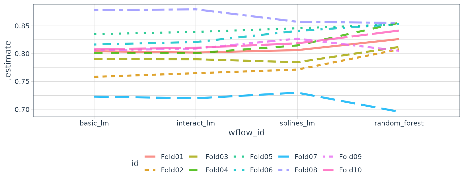
If there are no correlations within resamples, there would not be any parallel lines. Testing whether the correlations are significant:
> rsq_wider |>
  with(
    cor.test(
      basic_lm,
      splines_lm
    )
  ) |>
  tidy() |>
  select(
    estimate,
    starts_with("conf")
  )
# A tibble: 1 × 3
  estimate conf.low conf.high
     <dbl>    <dbl>     <dbl>
1    0.948    0.790     0.988
So why is this important? Consider the variance of a difference of two variables:
\[\begin{aligned} \text{var}(X - Y) &= \text{var}(X) + \text{var}(Y) - 2\text{cov}(X, Y) \end{aligned}\]Hence, if there is a significant positive covariance, then any statistical test of the difference would be reduced.
Simple Hypothesis Testing Methods
With the ANOVA model, the predictors are binary dummy variables for different groups. The \(\beta\) parameters estimate whether two or more groups are different from one another:
Supposed the outcome \(y_{ij}\) are the individual resample \(R^{2}\) statistics and X1, X2, and X3 columns are indicators for the models:
\[\begin{aligned} y_{ij} &= \beta_{0} + \beta_{1}x_{i1} + \beta_{2}x_{i2} + \beta_{p}x_{i3} + e_{ij} \end{aligned}\]- \(\beta_{0}\) is the mean \(R^{2}\) statistic for the basic linear models
- \(\beta_{1}\) is the change in the mean \(R^{2}\) statistic when interactions are added to the basic linear model
- \(\beta_{1}\) is the change in the mean \(R^{2}\) statistic between basic linear model and random forest model
- \(\beta_{1}\) is the change in the mean \(R^{2}\) statistic between basic linear model and model with interactions and splines
However, we still need to contend with how to handle the re-sample-to-resample effect. However, when considering two models at a time, the outcomes are matched by resample and the differences do not contain the resample-to-resample effect:
compare_lm <- rsq_wider |>
  mutate(
    difference = splines_lm - basic_lm
  )
> compare_lm
# A tibble: 10 × 6
   id     random_forest basic_lm interact_lm splines_lm difference
   <chr>          <dbl>    <dbl>       <dbl>      <dbl>      <dbl>
 1 Fold01         0.859    0.848       0.847      0.850    0.00186
 2 Fold02         0.837    0.802       0.808      0.822    0.0195
 3 Fold03         0.869    0.842       0.846      0.848    0.00591
 4 Fold04         0.819    0.791       0.789      0.795    0.00319
 5 Fold05         0.817    0.821       0.825      0.832    0.0106
 6 Fold06         0.825    0.807       0.811      0.830    0.0232
 7 Fold07         0.825    0.795       0.795      0.792   -0.00363
 8 Fold08         0.767    0.737       0.737      0.745    0.00760
 9 Fold09         0.835    0.780       0.778      0.791    0.0108
10 Fold10         0.807    0.786       0.791      0.802    0.0153

> lm(
  difference ~ 1,
  data = compare_lm
) |>
  tidy(conf.int = TRUE) |>
  select(
    estimate,
    p.value,
    starts_with("conf")
  )
# A tibble: 1 × 4
  estimate p.value conf.low conf.high
     <dbl>   <dbl>    <dbl>     <dbl>
1  0.00944 0.00554  0.00355    0.0153
A Random Intercept Model (Bayesian Method)
Historically, the resample groups are considered block effect and an appropriate term is added to the model. Alternatively, the resample effect could be considered a random effect where the resamples were drawn at random from a larger population of possible models. Methods for fitting an ANOVA model with this type of random effect are Linear Mixed Model or a Bayesian Hierarchical Model.
The ANOVA model assumes the errors \(e_{ij}\) to be independent and follow a Gaussian distribution \(N(0, \sigma)\). A Bayesian linear model makes additional assumptions, We specify a prior distribution for the model parameters. For example a fairly uninformative priors:
\[\begin{aligned} e_{ij} &\sim N(0, \sigma)\\ \beta_{j} &\sim N(0, 10)\\ \sigma &\sim \text{Exp}(1) \end{aligned}\]To adapt the ANOVA model so that the resamples are adequately modeled, we consider a random intercept model. We assume that the resamples impact the only through the intercept and that the regression parameters \(\beta_{j}\) have the same relationship across resamples.
\[\begin{aligned} y_{ij} &= (\beta_{0} + b_{i}) + \beta_{1}x_{i1} + \beta_{2}x_{i2} + \beta_{p}x_{i3} + e_{ij} \end{aligned}\]And we assume the following prior for \(b_{i}\):
\[\begin{aligned} b_{i} &\sim t(1) \end{aligned}\]The perf_mod() in tidyposterior package can be used for comparing resampled models. For workflow sets, it creates an ANOVA model where the groups correspond to the workflows. If one of the workflows in the set had tunng parameters, the best tuning parameters set for each workflow will be used in the Bayesian analysis. In this case, perf_mode() focuses on between-workflow comparisons.
For objects that contain a single model and tuned using resampling, perf_mod() makes within-model comparisons. In this case, the Bayesian ANOVA model groups the submodels defined by the tuning parameters.
perf_mod() uses default priors for all parameters except for the random intercepts which we would need to specify.
rsq_anova <- perf_mod(
  four_models,
  metric = "rsq",
  prior_intercept = rstanarm::student_t(df = 1),
  chains = 4,
  iter = 5000,
  seed = 1102
)

> rsq_anova
Bayesian Analysis of Resampling Results
Original data: 10-fold cross-validation
Next we take random samples from the posterior distribution:
model_post <- rsq_anova |>
  tidy(seed = 1103)

> model_post
# Posterior samples of performance
# A tibble: 40,000 × 2
   model         posterior
   <chr>             <dbl>
 1 random_forest     0.837
 2 basic_lm          0.806
 3 interact_lm       0.808
 4 splines_lm        0.817
 5 random_forest     0.830
 6 basic_lm          0.806
 7 interact_lm       0.811
 8 splines_lm        0.818
 9 random_forest     0.826
10 basic_lm          0.796
# ℹ 39,990 more rows
# ℹ Use `print(n = ...)` to see more rows
Plotting the 3 posterior distributions from the random samples:
model_post |>
  mutate(
    model = forcats::fct_inorder(model)
  ) |>
  ggplot(aes(x = posterior)) +
  geom_histogram(
    bins = 50,
    color = "white",
    fill = "blue",
    alpha = 0.4
  ) +
  facet_wrap(
    ~model,
    ncol = 1
  ) +
  theme_tq()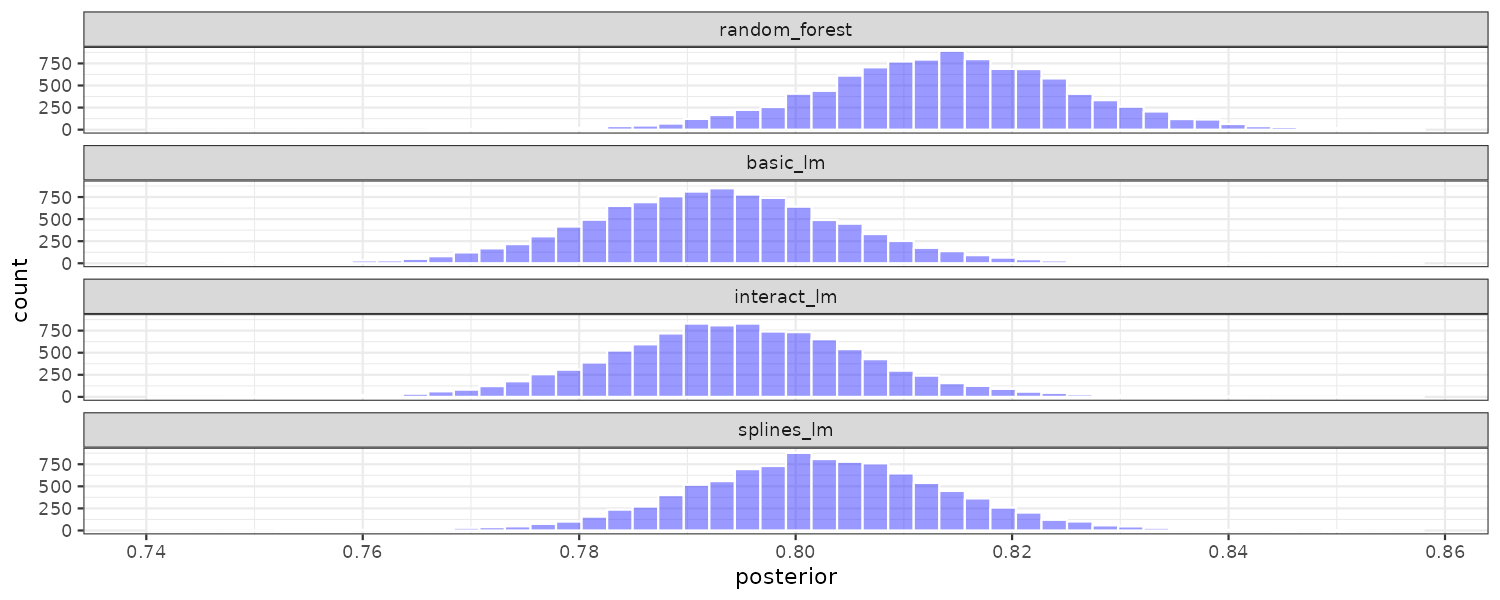
Or we could call autoplot() directly on the perf_mod() object:
autoplot(rsq_anova) +
  geom_text_repel(
    aes(label = workflow),
    nudge_x = 1 / 8,
    nudge_y = 1 / 100
  ) +
  theme(legend.position = "none") +
  theme_tq()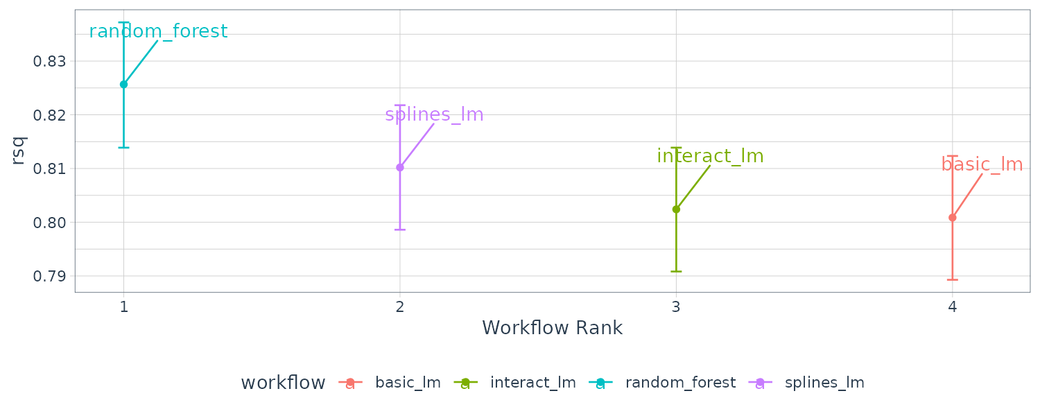
Once we have the posterior distribution for the parameters, it is trivial to get the posterior distributions for combinations of the parameters. For example, the contrast_models() can compare the differences between models:
rqs_diff <- contrast_models(
  rsq_anova,
  list_1 = "splines_lm",
  list_2 = "basic_lm",
  seed = 1104
)

> rqs_diff
# Posterior samples of performance differences
# A tibble: 10,000 × 4
   difference model_1    model_2  contrast
        <dbl> <chr>      <chr>    <chr>
 1    0.0111  splines_lm basic_lm splines_lm vs. basic_lm
 2    0.0119  splines_lm basic_lm splines_lm vs. basic_lm
 3    0.0136  splines_lm basic_lm splines_lm vs. basic_lm
 4    0.00412 splines_lm basic_lm splines_lm vs. basic_lm
 5    0.00402 splines_lm basic_lm splines_lm vs. basic_lm
 6    0.0116  splines_lm basic_lm splines_lm vs. basic_lm
 7    0.00482 splines_lm basic_lm splines_lm vs. basic_lm
 8    0.0136  splines_lm basic_lm splines_lm vs. basic_lm
 9    0.0124  splines_lm basic_lm splines_lm vs. basic_lm
10    0.0118  splines_lm basic_lm splines_lm vs. basic_lm
# ℹ 9,990 more rows
# ℹ Use `print(n = ...)` to see more rows
And plotting the difference histogram:
rqs_diff |>
  as_tibble() |>
  ggplot(aes(x = difference)) +
  geom_vline(
    xintercept = 0,
    lty = 2
  ) +
  geom_histogram(
    bins = 50,
    color = "white",
    fill = "red",
    alpha = 0.4
  ) +
  theme_tq()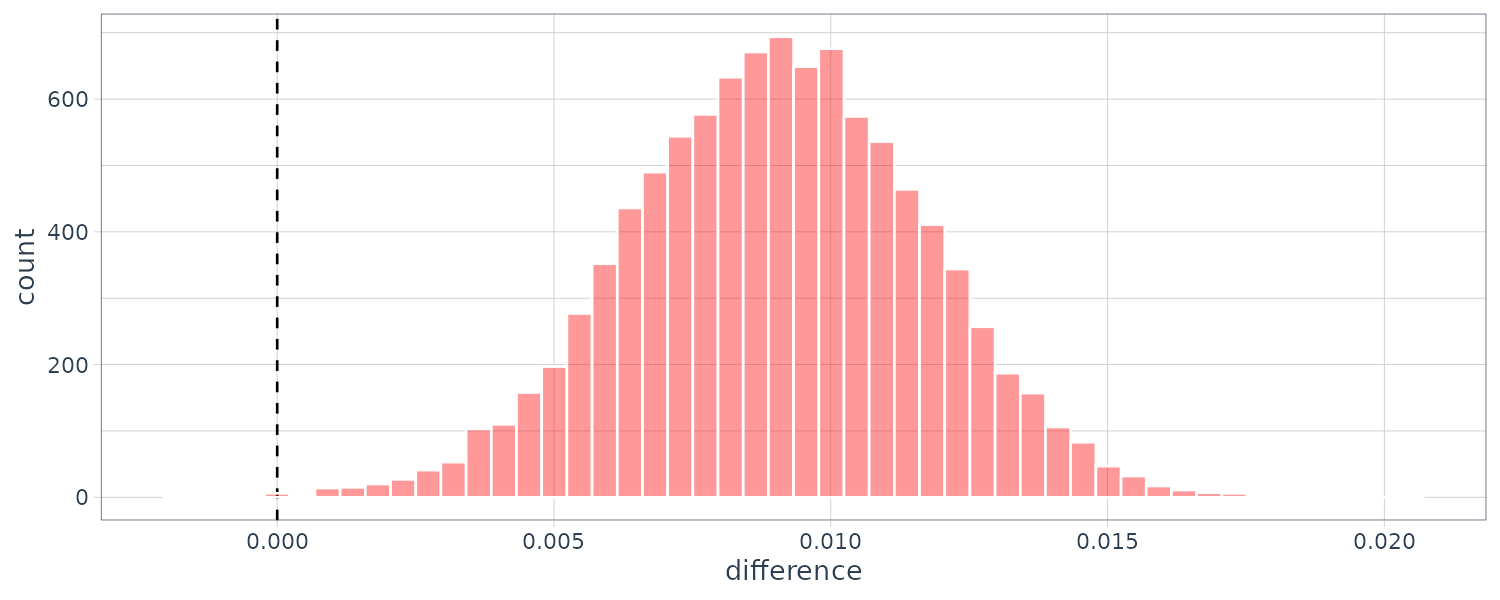
The summary() method computes the credible intervals as well as a probability column that the proportion of the posterior is greater than 0.
> summary(rqs_diff) |>
  select(-starts_with("pract"))
# A tibble: 1 × 6
  contrast               probability    mean   lower  upper  size
  <chr>                        <dbl>   <dbl>   <dbl>  <dbl> <dbl>
1 splines_lm vs basic_lm       0.999 0.00902 0.00465 0.0133     0
Although statistically significant, the mean is too low to be practical. To check for practical significance of 2%, we can employ the Region of Practical Equivalence (ROPE) estimate, the size option of the summary function is used:
> summary(
  rqs_diff,
  size = 0.02
) |>
  select(
    contrast,
    starts_with("pract")
  )
# A tibble: 1 × 4
  contrast               pract_neg pract_equiv pract_pos
  <chr>                      <dbl>       <dbl>     <dbl>
1 splines_lm vs basic_lm         0        1.00    0.0001
The pract_equiv column is the proportion of the posterior that is within [-size, size]. pract_neg and pract_pos are proportions below and above this interval. As we can see, the mean is not practically significant.
The autoplot() method can show the pract_equiv results that compare each workflow to the current best (the random forest model, in this case which is 1):
autoplot(
  rsq_anova,
  type = "ROPE",
  size = 0.02
) +
  geom_text_repel(aes(label = workflow)) +
  theme(legend.position = "none") +
  theme_tq()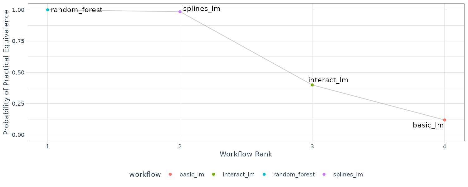
Model Tuning
Parameters that cannot be directly estimated from the training data but specified ahead of time are called hyperparmeters or tuning parameters.
Some examples of tuning paramaters are:
Boosting
Boosting is an ensemble model that combines a series of base models that are created sequentially and each model is dependent on the previous models. The number of boosting iterations is a tuning parameter.
Multilayer Perceptron
Also known as the single-layer aritifical neural network. The hidden units are linear combinations of the predictors that are feed into a activation function such as a sigmoid. The number of hidden units and type of activation functions can be tuned.
Gradient Descent
Gradient descent parameters such as the learning rates, momentum, and the number of optimazation iterations/epochs can be tuned.
PCA
The number of principal components to be used can be tuned.
Imputation by K-Nearest Neighbors
The number of neighbors can be tuned.
Logistic Regression
The logit link function (such as logit, probit, and complementary log-log) can be tuned.
But note that we should never tune a parameter in the prior distribution for Bayesian analysis as that will defeat the purpose of a prior distribution.
Likelihoods
But what criteria do we optimize? For cases where the statistical properties of the tuning parameter are tractable, we can maximize the likelihood or information criteria. Note that these statistical properties may not align with the results achieved using accuracy-oriented properties.
Consider fitting a logistic regression model to the iris dataset. We would like to optimize the link function. The three link functions in considerations are logit, probit, and the complementary log-log model.
\[\begin{aligned} \log\Big(\frac{\pi}{1 - \pi}\Big) &= \beta_{0} + \beta_{1}x_{1} + \cdots + \beta_{p}x_{p}\\[5pt] \Phi^{-1}(\pi) &= \beta_{0} + \beta_{1}x_{1} + \cdots + \beta_{p}x_{p}\\[5pt] \log(-\log(1 - \pi)) &= \beta_{0} + \beta_{1}x_{1} + \cdots + \beta_{p}x_{p}\\ \end{aligned}\]The statistical approach is to compute the log-likelihood for each model and choose the model with the largest value. Traditionally, the likelihood is computed from the training data.
Let’s create a function to extract the likelihood from fitting the model:
training_set <- iris |>
  filter(Species %in% c("setosa", "virginica"))
training_set$Species <- factor(training_set$Species)
training_set <- tibble(training_set)

llhood <- function(...) {
  logistic_reg() |>
    set_engine("glm", ...) |>
    fit(
      Species ~ .,
      data = training_set) |>
    glance() |>
    select(logLik)
}

> bind_rows(
  llhood(),
  llhood(family = binomial(link = "probit")),
  llhood(family = binomial(link = "cloglog"))
) |>
  mutate(
    link = c("logit", "probit", "c-log-log")
  ) |>
  arrange(desc(logLik))
# A tibble: 3 × 2
     logLik link
      <dbl> <chr>
1 -2.59e-10 probit
2 -4.29e-10 logit
3 -4.43e-10 c-log-log
According to the log-likelihood, the logit link function is the best.
But are the differences significant? We would need to see the confidence level as wel. We could resample the statistics. In the yardstick package, the mn_log_loss() function is used to estimate the negative log-likelihood:
set.seed(1201)
rs <- vfold_cv(
  training_set,
  repeats = 10
)

lloss <- function(...) {
  perf_meas <- metric_set(
    roc_auc,
    mn_log_loss
  )

  logistic_reg() |>
    set_engine(
      "glm",
      ...
    ) |>
    fit_resamples(
      Species ~ Sepal.Length,
      rs,
      metrics = perf_meas
    ) |>
    collect_metrics(summarize = FALSE) |>
    select(
      id,
      id2,
      .metric,
      .estimate
    )
}
Next we test it on the different link functions:
resampled_res <- bind_rows(
  lloss() |>
    mutate(
      model = "logistic"
    ),
  lloss(family = binomial(link = "probit")) |>
    mutate(
      model = "probit"
    ),
  lloss(family = binomial(link = "cloglog")) |>
    mutate(
      model = "c-log-log"
    )
) |>
  # Convert log-loss to log-likelihood:
  mutate(.estimate = ifelse(
    .metric == "mn_log_loss",
    -.estimate,
    .estimate
  )) |>
  group_by(model, .metric) |>
  summarize(
    mean = mean(.estimate, na.rm = TRUE),
    std_err = sd(.estimate, na.rm = TRUE) /
      sum(!is.na(.estimate)),
    .groups = "drop"
  )

> resampled_res
# A tibble: 6 × 4
  model     .metric       mean  std_err
  <chr>     <chr>        <dbl>    <dbl>
1 c-log-log mn_log_loss -0.174 0.00270
2 c-log-log roc_auc      0.984 0.000467
3 logistic  mn_log_loss -0.197 0.00333
4 logistic  roc_auc      0.984 0.000467
5 probit    mn_log_loss -0.314 0.00677
6 probit    roc_auc      0.984 0.000474
Let’s graph the confidence intervals for log-likelihood:
resampled_res |>
  filter(.metric == "mn_log_loss") |>
  ggplot(aes(x = mean, y = model)) +
  geom_point() +
  geom_errorbar(
    aes(
      xmin = mean - 1.64 * std_err,
      xmax = mean + 1.64 * std_err
    ),
    width = .1
  ) +
  labs(y = NULL, x = "log-likelihood") +
  theme_tq()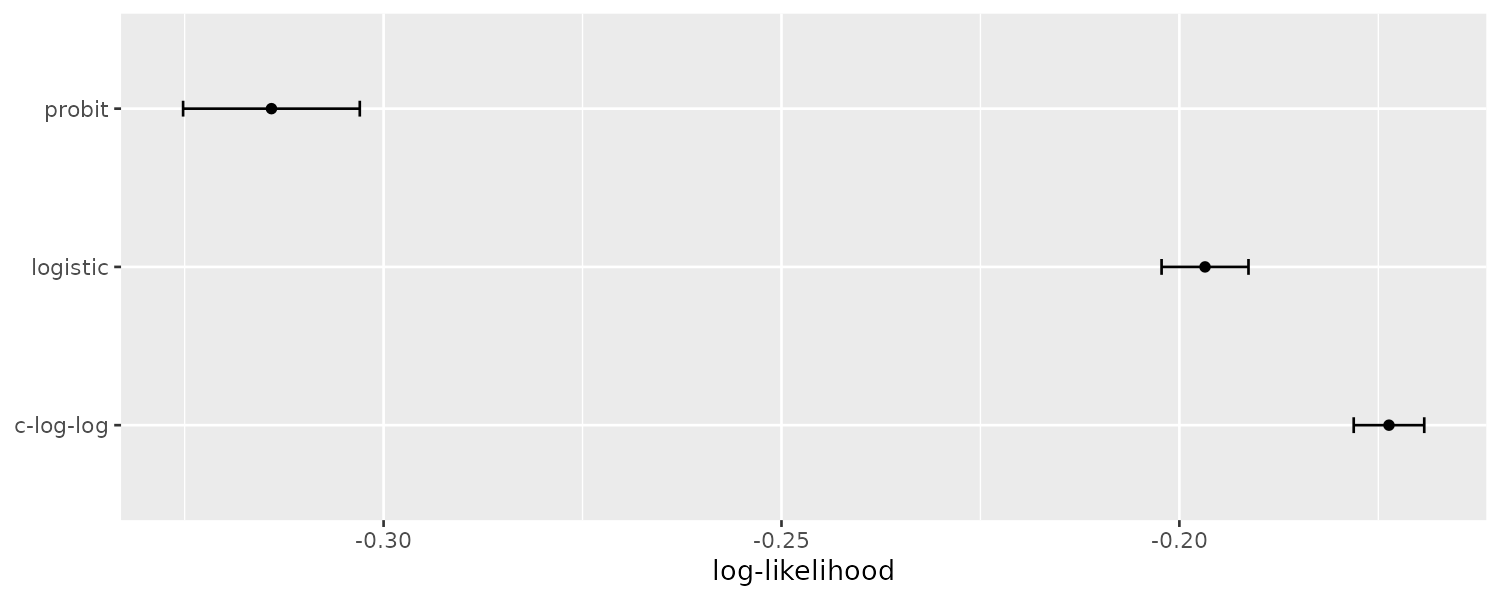
resampled_res |>
  filter(.metric == "roc_auc") |>
  ggplot(aes(x = mean, y = model)) +
  geom_point() +
  geom_errorbar(
    aes(
      xmin = mean - 1.64 * std_err,
      xmax = mean + 1.64 * std_err
    ),
    width = .1
  ) +
  labs(y = NULL, x = "roc area") +
  theme_tq()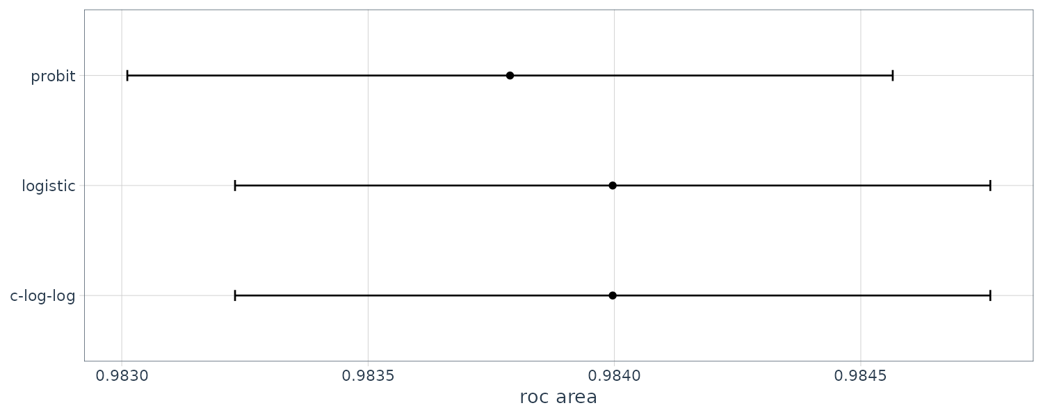
As we can see from the graphs, there is no difference in the AUC but considerable difference in terms of log-likelihoods.
Search Methods
Tuning parameters optimization falls into 2 categories:
Grid Search
The user predefine a set of parameter values to evaluate. An example would be the space-filling design.
Iterative Search
Also known as sequential search. New parameter combinations are based on previous results. Almost any nonlinear optimization method is appripriate, and in some cases, an initial set of results is required to start the optimization process. An example would be the Nelder-Mead simplex method.
Hybrid Search
After an initial grid search, a sequential optimization can start from the best grid combination.
Tuning Parameters in Parsnip Model Specification
There are two kind of parameter arguments in parsnip model specification. Main arguments are those that are most used in mulitple engines and engine specific parameters. For example, for the “rand_forest”” parsnip model, “trees”, and “min_n” are main parameters and “regularization.factor” is a secondary parameter:
rand_spec <- rand_forest(
  trees = 2000,
  min_n = tune()
) |>
  set_engine(
    "ranger",
    regularization.factor = tune()
  ) |>
  set_mode("regression")
We can use the extract_parameter_set_dials() function to enumerate the tuning parameters for a mlp object:
neural_net_spec <- mlp(
  hidden_units = tune()
) |>
  set_engine("keras") |>
  set_mode("regression")

extract_parameter_set_dials(neural_net_spec)
When both recipe and model specification are combined in a workflow, extract_parameter_set_dials will show both tuning parameters:
ames_rec <- recipe(
  Sale_Price ~ Neighborhood +
    Gr_Liv_Area +
    Year_Built +
    Bldg_Type +
    Latitude +
    Longitude,
  data = ames_train) |>
  step_log(Gr_Liv_Area, base = 10) |>
  step_other(Neighborhood, threshold = tune()) |>
  step_dummy(all_nominal_predictors()) |>
  step_interact(~ Gr_Liv_Area:starts_with("Bldg_Type_")) |>
  step_ns(Longitude, deg_free = tune("longitude df")) |>
  step_ns(Latitude, deg_free = tune("latitude df"))

> workflow() |>
  add_recipe(ames_rec) |>
  add_model(neural_net_spec) |>
  extract_parameter_set_dials()

Collection of 4 parameters for tuning

   identifier         type    object
 hidden_units hidden_units nparam[+]
    threshold    threshold nparam[+]
 longitude df     deg_free nparam[+]
  latitude df     deg_free nparam[+]
And to extract the range from a particular parameter object:
wflow_param <- workflow() |>
  add_recipe(ames_rec) |>
  add_model(rand_spec) |>
  extract_parameter_set_dials() |>
  update(threshold = threshold(c(0.8, 1.0)))

> wflow_param |>
  extract_parameter_dials("min_n")
Minimal Node Size (quantitative)
Range: [2, 40]

> wflow_param |>
  extract_parameter_dials("regularization.factor")
Gain Penalization (quantitative)
Range: [0, 1]

> wflow_param |>
  extract_parameter_dials("longitude df")
Spline Degrees of Freedom (quantitative)
Range: [1, 15]
Each tuning parameter argument has a corresponding function in the dials package that usually has the same name and gives the default range:
> threshold()
Threshold (quantitative)
Range: [0, 1]
> min_n()
Minimal Node Size (quantitative)
Range: [2, 40]
Some of them has a slight tweak in their names:
> regularization_factor()
Gain Penalization (quantitative)
Range: [0, 1]
> spline_degree()
Spline Degrees of Freedom (quantitative)
Range: [1, 10]
Some of the parameters do not have a default value until you use the finalize() function. For example, the following rspec would have a “?” in the “mtry” value because the algorithm doesn’t know the number of columns:
rf_spec <- rand_forest(mtry = tune()) |>
  set_engine(
    "ranger",
    regularization.factor = tune("regularization")) |>
  set_mode("regression")

rf_param <- extract_parameter_set_dials(rf_spec)

> rf_param
Collection of 2 parameters for tuning

     identifier                  type    object
           mtry                  mtry nparam[?]
 regularization regularization.factor nparam[+]

Model parameters needing finalization:
   # Randomly Selected Predictors ('mtry')

See `?dials::finalize` or `?dials::update.parameters` for more information.
The finalize() function can execute the recipe once to obtain the dimensions:
> rf_param |>
  finalize(ames_train) |>
  extract_parameter_dials("mtry")
# Randomly Selected Predictors (quantitative)
Range: [1, 74]
The range of the parameters can also be updated:
> wflow_param |>
  update(
    threshold = threshold(c(0.8, 1.0))
  ) |>
  extract_parameter_dials("threshold")
Threshold (quantitative)
Range: [0.8, 1]
But note that certain tuning parameters are associated with transformations. For example, the penalty parameter has a transformation by default (making sure the penalty is positive):
> penalty()
Amount of Regularization (quantitative)
Transformer: log-10 [1e-100, Inf]
Range (transformed scale): [-10, 0]

> penalty(c(-1, 0)) |>
  value_sample(1000) |>
  summary()
   Min. 1st Qu.  Median    Mean 3rd Qu.    Max.
 0.1000  0.1843  0.3133  0.3833  0.5415  0.9970

> penalty(c(0.1, 1.0)) |>
  value_sample(1000) |>
  summary()
   Min. 1st Qu.  Median    Mean 3rd Qu.    Max.
  1.262   2.218   3.585   4.255   5.853   9.958
As you can see from above, the penalty is being transformed. In order to pass in transformed range:
> penalty(
  trans = NULL,
  range = 10^c(-10, 0)
)
Amount of Regularization (quantitative)
Range: [1e-10, 1]
Grid Search
Grid search is when we predefine a set of parameter values to evaluate. The parameter space can become unmanageable because of the curse of dimensionality.
We will consider a multilayer perceptron model with the following tuning parameters:
- number of hidden units
- number of epochs/iterations
- amount of weight decay penalization
mlp_spec <- mlp(
  hidden_units = tune(),
  penalty = tune(),
  epochs = tune()
) |>
  set_engine("nnet", trace = 0) |>
  set_mode("classification")

> mlp_spec
Single Layer Neural Network Model Specification (classification)

Main Arguments:
  hidden_units = tune()
  penalty = tune()
  epochs = tune()

Engine-Specific Arguments:
  trace = 0

Computational engine: nnet

mlp_param <- extract_parameter_set_dials(mlp_spec)

> mlp_param |>
  extract_parameter_dials("hidden_units")
# Hidden Units (quantitative)
Range: [1, 10]

> mlp_param |>
  extract_parameter_dials("penalty")
Amount of Regularization (quantitative)
Transformer: log-10 [0.00....1, Inf]
Range (transformed scale): [-10, 0]

> mlp_param |>
  extract_parameter_dials("epochs")
# Epochs (quantitative)
Range: [10, 1000]
Regular Grids
The crossing() function is one way to create a regular grid:
> crossing(
  hidden_units = 1:3,
  penalty = c(0.0, 0.1),
  epochs = c(100, 200)
)
# A tibble: 12 × 3
   hidden_units penalty epochs
          <int>   <dbl>  <dbl>
 1            1     0      100
 2            1     0      200
 3            1     0.1    100
 4            1     0.1    200
 5            2     0      100
 6            2     0      200
 7            2     0.1    100
 8            2     0.1    200
 9            3     0      100
10            3     0      200
11            3     0.1    100
12            3     0.1    200
Or using grid_*() functions:
> mlp_param |>
  grid_regular(levels = 2)
# A tibble: 8 × 3
  hidden_units      penalty epochs
         <int>        <dbl>  <int>
1            1 0.0000000001     10
2           10 0.0000000001     10
3            1 1                10
4           10 1                10
5            1 0.0000000001   1000
6           10 0.0000000001   1000
7            1 1              1000
8           10 1              1000
The levels argument can also take a named vector of values:
> mlp_param |>
  grid_regular(
    levels = c(
      hidden_units = 3,
      penalty = 2,
      epochs = 2
    )
  )
# A tibble: 12 × 3
   hidden_units      penalty epochs
          <int>        <dbl>  <int>
 1            1 0.0000000001     10
 2            5 0.0000000001     10
 3           10 0.0000000001     10
 4            1 1                10
 5            5 1                10
 6           10 1                10
 7            1 0.0000000001   1000
 8            5 0.0000000001   1000
 9           10 0.0000000001   1000
10            1 1              1000
11            5 1              1000
12           10 1              1000
Nonregular Grids
The grid_random() function generates independent uniform random numbers across parameter ranges:
> mlp_param |>
  grid_random(size = 1000)
# A tibble: 1,000 × 3
   hidden_units       penalty epochs
          <int>         <dbl>  <int>
 1            4 0.168             29
 2            2 0.00000768       678
 3           10 0.0000000311     232
 4            2 0.0000000392     648
 5            4 0.0000000334     679
 6            6 0.00000000471    593
 7           10 0.0189           472
 8            9 0.00799          748
 9            9 0.00000340       525
10            2 0.000441          64
# ℹ 990 more rows
# ℹ Use `print(n = ...)` to see more rows
The problem with grid_random() is the potential of overlapping parameter combinations. For example, rows with the same hidden_units value.
A better approach is using a type of experimental design called space-filling designs that minimizing overlapping combinations and space the points farther apart from each other. The default design is the maximum entropy design.
> mlp_param |>
  grid_latin_hypercube(
    size = 20,
    original = FALSE
  )
# A tibble: 20 × 3
   hidden_units penalty epochs
          <dbl>   <dbl>  <dbl>
 1         9.68 -0.960   644.
 2         3.71 -5.22    905.
 3         7.89 -4.68    461.
 4         7.25 -6.38    697.
 5         9.26 -3.86    131.
 6         3.20 -3.44     59.7
 7         5.85 -1.04    452.
 8         1.38 -7.12     34.2
 9         4.46 -0.0734  542.
10         8.92 -3.00    852.
11         6.08 -9.96    980.
12         3.59 -7.85    579.
13         1.73 -8.70    395.
14         2.22 -4.31    767.
15         5.49 -6.78    267.
16         7.33 -9.16    742.
17         2.42 -8.06    826.
18         6.68 -5.56    321.
19         8.34 -2.30    191.
20         5.00 -1.51    209.
Evaluating the Grid
To choose the best tuning parameter combination, each candidate set is tested on data that were not used in the model. Resapling or a validation set can be used for this purpose.
In this example, we will use the “cell” dataset which consists of 56 imaging measurements on 2,019 human breast cancer cells. The predictors represent shape and intensity characteristics of different parts of the cells (e.g., the nucleus, the cell boundary, etc.). Each cell belongs to one of two classes (PS vs WS). There is a high correlation between the predictors and many of the predictors have skewed distributions.
cells <- cells |>
  select(-case)

> cells
# A tibble: 2,019 × 57
   class angle_ch_1 area_ch_1
   <fct>      <dbl>     <int>
 1 PS        143.         185
 2 PS        134.         819
 3 WS        107.         431
 4 PS         69.2        298
 5 PS          2.89       285
 6 WS         40.7        172
 7 WS        174.         177
 8 PS        180.         251
 9 WS         18.9        495
10 WS        153.         384
# ℹ 2,009 more rows
# ℹ 54 more variables:
#   avg_inten_ch_1 <dbl>,
#   avg_inten_ch_2 <dbl>,
#   avg_inten_ch_3 <dbl>,
#   avg_inten_ch_4 <dbl>,
#   convex_hull_area_ratio_ch_1 <dbl>, …
# ℹ Use `print(n = ...)` to see more rows

set.seed(1304)
cell_folds <- vfold_cv(cells)
Due to the high correlation, we will use PCA and tune the number of components to keep. Yeo-Johnson transformation is to help in making more symmetric distributions due to the skewness. Two normalization is done because the lower-rank PCA components tend to have a wider range than the higher-rank components although technically they are on the same scale.
Note that in step_pca(), using zero PCA components is a shortcut to skip the feature extraction. In this way, resampling can include the original predictors and compared with results including PCA components.
mlp_spec <- mlp(
  hidden_units = tune(),
  penalty = tune(),
  epochs = tune()
) |>
  set_engine("nnet", trace = 0) |>
  set_mode("classification")

mlp_rec <- recipe(class ~ ., data = cells) |>
  step_YeoJohnson(all_numeric_predictors()) |>
  step_normalize(all_numeric_predictors()) |>
  step_pca(
    all_numeric_predictors(),
    num_comp = tune()
  ) |>
  step_normalize(all_numeric_predictors())

mlp_wflow <- workflow() |>
  add_model(mlp_spec) |>
  add_recipe(mlp_rec)
The default epoch ranges are too wide and num_comp range too low:
> mlp_wflow |>
  extract_parameter_dials("epochs")
# Epochs (quantitative)
Range: [10, 1000]

> mlp_wflow |>
  extract_parameter_dials("num_comp")
# Components (quantitative)
Range: [1, 4]
So let’s increase it:
mlp_param <- mlp_wflow |>
  extract_parameter_set_dials() |>
  update(
    epochs = epochs(c(50, 200)),
    num_comp = num_comp(c(0, 40))
  )
Let’s start the tuning. The interface to tune_grid() is similar to fit_resamples(). To start, we evaluate a regular grid with 3 levels:
roc_res <- metric_set(roc_auc)
set.seed(1305)
mlp_reg_tune <- mlp_wflow |>
  tune_grid(
    cell_folds,
    grid = mlp_param |>
      grid_regular(levels = 3),
    metrics = roc_res
  )

> mlp_reg_tune
# Tuning results
# 10-fold cross-validation
# A tibble: 10 × 4
   splits             id     .metrics
   <list>             <chr>  <list>
 1 <split [1817/202]> Fold01 <tibble>
 2 <split [1817/202]> Fold02 <tibble>
 3 <split [1817/202]> Fold03 <tibble>
 4 <split [1817/202]> Fold04 <tibble>
 5 <split [1817/202]> Fold05 <tibble>
 6 <split [1817/202]> Fold06 <tibble>
 7 <split [1817/202]> Fold07 <tibble>
 8 <split [1817/202]> Fold08 <tibble>
 9 <split [1817/202]> Fold09 <tibble>
10 <split [1818/201]> Fold10 <tibble>
# ℹ 1 more variable: .notes <list>
It is possible to graph the performance profiles across tuning parameters:
autoplot(mlp_reg_tune) +
  scale_color_viridis_d(direction = -1) +
  theme(legend.position = "top")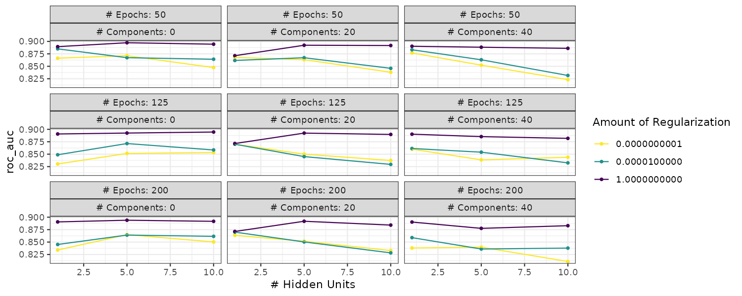
The number of epochs doesn’t seem to matter much to the AUC. The number of hidden units appears to matter when the amount of regularization penalty is low. When the penalty is high, the ROC across hidden units is pretty flat.
We can see the top 5 ranked performance:
> show_best(mlp_reg_tune) |>
  select(-.estimator) |>
  print(width = Inf)
# A tibble: 5 × 9
  hidden_units penalty epochs num_comp .metric  mean     n std_err .config
         <int>   <dbl>  <int>    <int> <chr>   <dbl> <int>   <dbl> <chr>
1            5       1    125        0 roc_auc 0.897    10 0.00705 Preprocessor1_Model17
2           10       1     50        0 roc_auc 0.897    10 0.00626 Preprocessor1_Model09
3            5       1     50       20 roc_auc 0.894    10 0.00543 Preprocessor2_Model08
4            5       1     50        0 roc_auc 0.893    10 0.00531 Preprocessor1_Model08
5           10       1    125       20 roc_auc 0.893    10 0.00681 Preprocessor2_Model18
To use a space-filling design, the grid argument can be given an integer value. For example, to evaluate the same range using a maximum entropy design with 20 candidate values:
set.seed(1306)
mlp_sfd_tune <- mlp_wflow |>
  tune_grid(
    cell_folds,
    grid = 20,
    param_info = mlp_param,
    metrics = roc_res
  )

> mlp_sfd_tune
# Tuning results
# 10-fold cross-validation
# A tibble: 10 × 4
   splits             id     .metrics          .notes
   <list>             <chr>  <list>            <list>
 1 <split [1817/202]> Fold01 <tibble [20 × 8]> <tibble [0 × 3]>
 2 <split [1817/202]> Fold02 <tibble [20 × 8]> <tibble [0 × 3]>
 3 <split [1817/202]> Fold03 <tibble [20 × 8]> <tibble [0 × 3]>
 4 <split [1817/202]> Fold04 <tibble [20 × 8]> <tibble [0 × 3]>
 5 <split [1817/202]> Fold05 <tibble [20 × 8]> <tibble [0 × 3]>
 6 <split [1817/202]> Fold06 <tibble [20 × 8]> <tibble [0 × 3]>
 7 <split [1817/202]> Fold07 <tibble [20 × 8]> <tibble [0 × 3]>
 8 <split [1817/202]> Fold08 <tibble [20 × 8]> <tibble [0 × 3]>
 9 <split [1817/202]> Fold09 <tibble [20 × 8]> <tibble [0 × 3]>
10 <split [1818/201]> Fold10 <tibble [20 × 8]> <tibble [0 × 3]>
Because there is no fixed regular design, we can only graph the marginal effects plot via autoplot():
autoplot(mlp_sfd_tune) 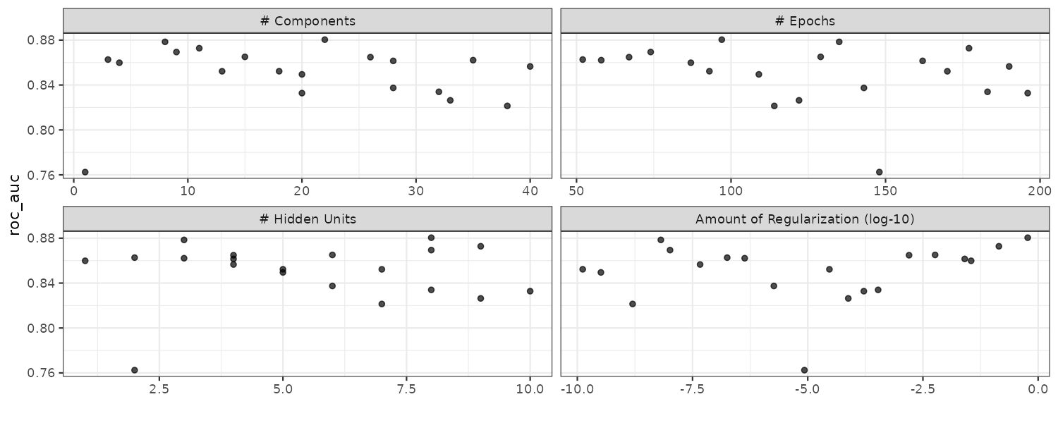
We can see the top 5 ranked performance:
> show_best(mlp_sfd_tune) |>
  select(-.estimator) |>
  print(width = Inf)
# A tibble: 5 × 9
  hidden_units       penalty epochs num_comp .metric  mean     n std_err .config
         <int>         <dbl>  <int>    <int> <chr>   <dbl> <int>   <dbl> <chr>
1            3 0.00000000649    135        8 roc_auc 0.879    10 0.00759 Preprocessor13_Model1
2            8 0.594             97       22 roc_auc 0.877    10 0.00920 Preprocessor16_Model1
3            9 0.141            177       11 roc_auc 0.872    10 0.00546 Preprocessor03_Model1
4            4 0.0255           162       28 roc_auc 0.866    10 0.00850 Preprocessor04_Model2
5            8 0.0000000103      74        9 roc_auc 0.865    10 0.00855 Preprocessor10_Model1
Note the contrasting result from the regular grids. Generally, it is a good idea to evaluate the models over multiple metrics and better to choose a slightly suboptimal but simpler model. In this case, would be a larger penalty values with fewer hidden units.
To save intermediary values in tunegrid(), use the extract option to control_grid and setting the save_pred to TRUE.
mlp_sfd_tune <- mlp_wflow |>
  tune_grid(
    cell_folds,
    grid = 20,
    param_info = mlp_param,
    metrics = roc_res,
    control = control_resamples(
      save_pred = TRUE,
      save_workflow = TRUE
    )
  )

> collect_predictions(mlp_sfd_tune)
# A tibble: 40,380 × 10
   id     .pred_PS .pred_WS  .row num_comp hidden_units   penalty epochs class .config
   <chr>     <dbl>    <dbl> <int>    <int>        <int>     <dbl>  <int> <fct> <chr>
 1 Fold01    0.555    0.445    14       34            7 0.0000108     51 PS    Preprocessor01_Model1
 2 Fold01    0.731    0.269    34       34            7 0.0000108     51 PS    Preprocessor01_Model1
 3 Fold01    0.729    0.271    42       34            7 0.0000108     51 PS    Preprocessor01_Model1
 4 Fold01    0.729    0.271    43       34            7 0.0000108     51 PS    Preprocessor01_Model1
 5 Fold01    0.731    0.269    96       34            7 0.0000108     51 PS    Preprocessor01_Model1
 6 Fold01    0.479    0.521   101       34            7 0.0000108     51 PS    Preprocessor01_Model1
 7 Fold01    0.731    0.269   106       34            7 0.0000108     51 PS    Preprocessor01_Model1
 8 Fold01    0.481    0.519   108       34            7 0.0000108     51 PS    Preprocessor01_Model1
 9 Fold01    0.385    0.615   118       34            7 0.0000108     51 WS    Preprocessor01_Model1
10 Fold01    0.729    0.271   122       34            7 0.0000108     51 PS    Preprocessor01_Model1
# ℹ 40,370 more rows
# ℹ Use `print(n = ...)` to see more rows
Finalizing the Model
To replace all the tune parameters with the best result from tuning:
best_param <- select_best(
  mlp_reg_tune,
  metric = "roc_auc"
)

final_mlp_wflow <- mlp_wflow |>
  finalize_workflow(best_param)
> final_mlp_wflow
══ Workflow ════════════════════════════════════════════════════
Preprocessor: Recipe
Model: mlp()

── Preprocessor ────────────────────────────────────────────────
4 Recipe Steps

• step_YeoJohnson()
• step_normalize()
• step_pca()
• step_normalize()

── Model ───────────────────────────────────────────────────────
Single Layer Neural Network Model Specification (classification)

Main Arguments:
  hidden_units = 5
  penalty = 1
  epochs = 50

Engine-Specific Arguments:
  trace = 0

Computational engine: nnet
And fitting a model to the entire training set:
final_mlp_fit <- final_mlp_wflow |>
  fit(cells)
Note there are different finalize functions depending on whether one is using a workflow, model or recipe:
- finalize_workflow()
- finalize_model()
- finalize_recipe()
Tools for Creating Tuning Specifications
The “usemodels” package is able to produce R code for tuning the model given just the dataframe and model formula. For example:
library(usemodels)

> use_xgboost(
  Sale_Price ~ Neighborhood +
    Gr_Liv_Area +
    Year_Built +
    Bldg_Type +
    Latitude +
    Longitude,
  data = ames_train,
  verbose = TRUE
)

xgboost_recipe <-
  recipe(formula = Sale_Price ~ Neighborhood + Gr_Liv_Area + Year_Built + Bldg_Type +
    Latitude + Longitude, data = ames_train) %>%
  step_zv(all_predictors())

xgboost_spec <-
  boost_tree(trees = tune(), min_n = tune(), tree_depth = tune(), learn_rate = tune(),
    loss_reduction = tune(), sample_size = tune()) %>%
  set_mode("classification") %>%
  set_engine("xgboost")

xgboost_workflow <-
  workflow() %>%
  add_recipe(xgboost_recipe) %>%
  add_model(xgboost_spec)

set.seed(7019)
xgboost_tune <-
  tune_grid(
    xgboost_workflow,
    resamples = stop("add your rsample object"),
    grid = stop("add number of candidate points")
  )
Parallel Processing
There are 2 type of parallelization strategy in tune functions via the argument “parallel_over””. The default argument is “resamples”. Each fold would only do the preprocessing once, but would do multiple tuning combinations per worker as the number of workers needed cannot exceed the number of folds.
The other argument is “everything”. This would replicate processing multiple times per worker, but tuning combinations can be assigned to multiple workers.
Access to Global Variables
When you pass a variable defined in the global environment, it could cause problem when running in parallel with parsnip. It is better to pass them as value rather than reference by using the !! operator.
coef_penalty <- 0.1
spec <- linear_reg(penalty = coef_penalty) |>
  set_engine("glmnet")

> spec$args$penalty
<quosure>
expr: ^coef_penalty
env:  global

spec <- linear_reg(penalty = !!coef_penalty) |>
  set_engine("glmnet")

> spec$args$penalty
<quosure>
expr: ^0.1
env:  empty
When you have more than one value, use the !!! operator:
mcmc_args <- list(
  chains = 3,
  iter = 1000,
  cores = 3
)
linear_reg() |>
  set_engine("stan", !!!mcmc_args)
Racing Methods
Some tuning parameters might give bad metrics in a number of resamplings, and dropped out totally in the subsequent resamples. This is known as racing methods.
The finetune package contains functions for racing (mirrors tune_grid):
mlp_sfd_race <- mlp_wflow |>
  tune_race_anova(
    cell_folds,
    grid = 20,
    param_info = mlp_param,
    metrics = roc_res,
    control = control_race(verbose_elim = TRUE)
  )

> mlp_sfd_race
# Tuning results
# 10-fold cross-validation
# A tibble: 10 × 5
   splits             id     .order .metrics          .notes
   <list>             <chr>   <int> <list>            <list>
 1 <split [1817/202]> Fold04      3 <tibble [20 × 8]> <tibble [0 × 3]>
 2 <split [1817/202]> Fold06      2 <tibble [20 × 8]> <tibble [0 × 3]>
 3 <split [1817/202]> Fold07      1 <tibble [20 × 8]> <tibble [0 × 3]>
 4 <split [1817/202]> Fold02      4 <tibble [9 × 8]>  <tibble [0 × 3]>
 5 <split [1817/202]> Fold08      5 <tibble [7 × 8]>  <tibble [0 × 3]>
 6 <split [1818/201]> Fold10      6 <tibble [5 × 8]>  <tibble [0 × 3]>
 7 <split [1817/202]> Fold01      7 <tibble [4 × 8]>  <tibble [0 × 3]>
 8 <split [1817/202]> Fold05      8 <tibble [3 × 8]>  <tibble [0 × 3]>
 9 <split [1817/202]> Fold09      9 <tibble [2 × 8]>  <tibble [0 × 3]>
10 <split [1817/202]> Fold03     10 <tibble [2 × 8]>  <tibble [0 × 3]>
show_best() returns the best models but returns only the configurations that were never elminated. Note less than 10 got returned:
> show_best(mlp_sfd_race)
# A tibble: 2 × 10
  hidden_units  penalty epochs num_comp .metric .estimator  mean     n std_err .config
         <int>    <dbl>  <int>    <int> <chr>   <chr>      <dbl> <int>   <dbl> <chr>
1            2 0.608       110       20 roc_auc binary     0.888    10 0.00649 Preprocessor12_Model1
2            6 0.000788     86        8 roc_auc binary     0.880    10 0.00  755 Preprocessor02_Model1
Iterative Search
Also known as sequential search. Parameter combinations are discovered sequentially based on previous results.
We are going to use a SVM model and the cell dataset to demonstrate iterative search. The two tuning parameters are the SVM cost value and the RBF kernel parameter \(\sigma\). The workflow and tuning spec are:
svm_rec <- recipe(class ~ ., data = cells) |>
  step_YeoJohnson(all_numeric_predictors()) |>
  step_normalize(all_numeric_predictors())

svm_spec <- svm_rbf(
  cost = tune(),
  rbf_sigma = tune()
) |>
  set_engine("kernlab") |>
  set_mode("classification")

svm_wflow <- workflow() |>
  add_model(svm_spec) |>
  add_recipe(svm_rec)
To improve the visualization of the search, we will narrow down the kernel parameter range:
svm_param <- svm_wflow |>
  extract_parameter_set_dials() |>
  update(rbf_sigma = rbf_sigma(c(-7, -1)))
Bayesian Optimization
Bayesian optimization techniques analyze the current resampling results and create a predictive model to suggest tuning parameter values. The suggested parameter combination is then resampled and the cycle follows.
Bayesian optimization analyze the current resampling results and create a surrogate predictive model to approximate the underlying unknown blackbox function (ROC vs cost + sigma), and suggesting tuning parameter values via an acquisition function.
We first address the surrogate function which we would use a Gaussian process model. Gaussian process models are specificed by mean and covariance functions. The covariance will be make up of RBF basis kernel functions. The nature of covariance function is as the distance between two tuning parameter combination increases, the covariance will increase exponentially.
A class of acquisition functions (Exploration vs Exploitation) facilitate the trade-off between mean and variance. Exploration biases toward higher variance region while Exploitation biases toward region that are closer to existing results. “Expected Improvement” is one of the commonly used acquisition functions. A higher variance region would tend to give a higher expected improvement. Another would be the confidence level approach. This is done by funding the tuning parameter combination associated with the largest confidence interval.
Given a starting initial param region:
set.seed(1401)
start_grid <- svm_param |>
  update(
    cost = cost(c(-6, 1)),
    rbf_sigma = rbf_sigma(c(-6, -4))
  ) |>
  grid_regular(levels = 2)

set.seed(1402)
roc_res <- metric_set(roc_auc)
svm_initial <- svm_wflow |>
  tune_grid(
    resamples = cell_folds,
    grid = start_grid,
    metrics = roc_res
  )

> collect_metrics(svm_initial)
# A tibble: 4 × 8
    cost rbf_sigma .metric .estimator  mean     n std_err .config
   <dbl>     <dbl> <chr>   <chr>      <dbl> <int>   <dbl> <chr>
1 0.0156  0.000001 roc_auc binary     0.865    10 0.00759 Preprocessor1_Model1
2 2       0.000001 roc_auc binary     0.863    10 0.00757 Preprocessor1_Model2
3 0.0156  0.0001   roc_auc binary     0.863    10 0.00763 Preprocessor1_Model3
4 2       0.0001   roc_auc binary     0.867    10 0.00709 Preprocessor1_Model4
Using the initial regular grid search, we continue with the Gaussian process model using the tune_bayes() function:
ctrl <- control_bayes(verbose = TRUE)
set.seed(1403)
svm_bo <- svm_wflow |>
  tune_bayes(
    resamples = cell_folds,
    metrics = roc_res,
    initial = svm_initial,
    param_info = svm_param,
    iter = 25,
    control = ctrl
  )

> show_best(svm_bo)
# A tibble: 5 × 9
   cost rbf_sigma .metric .estimator  mean     n std_err .config .iter
  <dbl>     <dbl> <chr>   <chr>      <dbl> <int>   <dbl> <chr>   <int>
1 31.2    0.00124 roc_auc binary     0.900    10 0.00610 Iter12     12
2 31.5    0.00127 roc_auc binary     0.900    10 0.00606 Iter17     17
3 31.9    0.00149 roc_auc binary     0.900    10 0.00617 Iter7       7
4 27.7    0.00145 roc_auc binary     0.899    10 0.00601 Iter11     11
5  4.46   0.00600 roc_auc binary     0.899    10 0.00645 Iter22     22
The autoplot() shows how the outcome changed over the search:
autoplot(svm_bo, type = "performance") 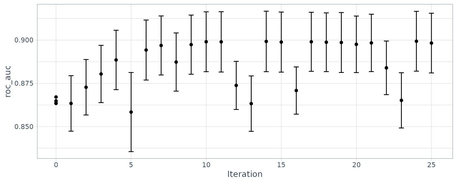
And also the parameter values over iterations:
autoplot(svm_bo, type = "parameters") 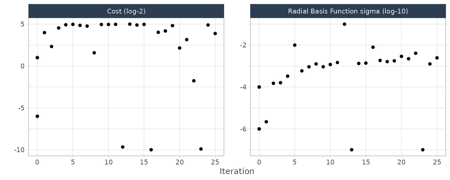
Note that rather than using a regular design for the initial grid, a space-filling design would probably be a better choice.
Simulated Annealing
The key distinguishing factor and unlike most graident-based optimization routines, simulated annleaing can reassess previous solutions. The process starts with an initial value and create a new candidate that is a small perturbation of the previous value.
The acceptance probability:
\[\begin{aligned} P(\text{accept parameters at iteration }i) &= e^{c \times D_{i} \times i}\\ i &= \text{iteration number}\\ c &= \text{constant}\\ D_{i} &= \% \text{ difference between the old and new values} \end{aligned}\]The probability is then compared to a random uniform number. If the acceptance probability is lower than the random uniform number, the search discards the current parameters and next iteration creates its candidate value in the neighborhood of its previous value. If not, the next iteration forms the next set of parameters based on current values.
The neighborhood is determined by scaling the current candidate to be between 0 and 1 based on the parameter range. Then radius values between 0.05 and 0.15 are considered. For nonnumeric parameters, we assign a probability for how often the parameter value changes.
To illustrate simulated annealing, we use the glmnet model and the following paramters tuning:
- Amount of total regularization (penalty)
- Proportion of the lasso penalty (mixture)
The process starts with the initial value of:
\[\begin{aligned} \text{penalty} &= 0.025\\ \text{mixture} &= 0.05 \end{aligned}\]The “no_improve” is an integer indicating the number of iterations that will continue if no improved results are discovered.
library(finetune)

ctrl_sa <- control_sim_anneal(
  verbose = TRUE,
  no_improve = 10L
)

set.seed(1404)

glmnet_rec <- recipe(class ~ ., data = cells) |>
  step_YeoJohnson(all_numeric_predictors()) |>
  step_normalize(all_numeric_predictors())

glmnet_spec <- logistic_reg(
  penalty = tune(),
  mixture = tune()
) |>
  set_engine("glmnet") |>
  set_mode("classification")

glmnet_wflow <- workflow() |>
  add_model(glmnet_spec) |>
  add_recipe(glmnet_rec)

glmnet_param <- glmnet_wflow |>
  extract_parameter_set_dials()

set.seed(1401)
roc_res <- metric_set(roc_auc)
glmnet_initial <- glmnet_wflow |>
  tune_grid(
    resamples = cell_folds,
    grid = data.frame(
      penalty = 0.025,
      mixture = 0.05
    ),
    metrics = roc_res
  )

> collect_metrics(glmnet_initial)
# A tibble: 1 × 8
  penalty mixture .metric .estimator  mean     n std_err .config
    <dbl>   <dbl> <chr>   <chr>      <dbl> <int>   <dbl> <chr>
1   0.025    0.05 roc_auc binary     0.881    10 0.00505 Preprocessor1_Model1
Running simulated annealing:
glmnet_sa <- glmnet_wflow |>
  tune_sim_anneal(
    resamples = cell_folds,
    metrics = roc_res,
    initial = glmnet_initial,
    param_info = glmnet_param,
    iter = 50,
    control = ctrl_sa
  )

> show_best(glmnet_sa)
# A tibble: 5 × 9
       penalty mixture .metric .estimator  mean     n std_err .config .iter
         <dbl>   <dbl> <chr>   <chr>      <dbl> <int>   <dbl> <chr>   <int>
1 0.0000274      0.804 roc_auc binary     0.895    10 0.00354 Iter49     49
2 0.00000384     0.800 roc_auc binary     0.895    10 0.00354 Iter48     48
3 0.00000429     0.660 roc_auc binary     0.894    10 0.00371 Iter39     39
4 0.0000301      0.532 roc_auc binary     0.894    10 0.00377 Iter41     41
5 0.0000000515   0.485 roc_auc binary     0.894    10 0.00378 Iter21     21
We can also plot the performance and the tuning parameters selection across iterations:
autoplot(glmnet_sa, type = "performance")
autoplot(glmnet_sa, type = "parameters")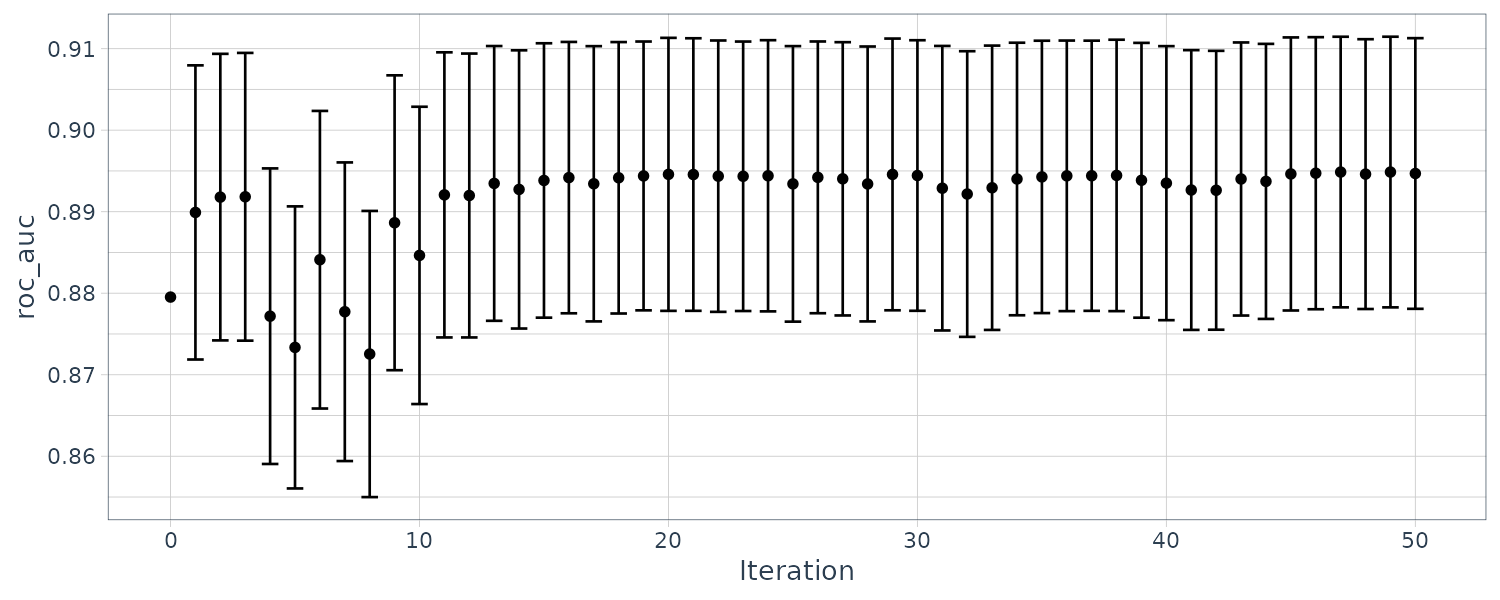
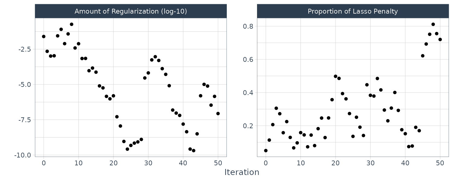
Screening Multiple Models
Workflow sets provide an interface to fit and compare multiple models. In this example we will use the concrete dataset, where we are predicting the compressive strength of concrete mixtures using ingredients as predictors.
data(concrete, package = "modeldata")

> concrete
# A tibble: 992 × 9
   cement blast_furnace_slag fly_ash water superplasticizer coarse_aggregate fine_aggregate   age compressive_strength
    <dbl>              <dbl>   <dbl> <dbl>            <dbl>            <dbl>          <dbl> <int>                <dbl>
 1   102                153        0  192                 0             887            942      3                 4.57
 2   102                153        0  192                 0             887            942      7                 7.68
 3   102                153        0  192                 0             887            942     28                17.3
 4   102                153        0  192                 0             887            942     90                25.5
 5   108.               162.       0  204.                0             938.           849      3                 2.33
 6   108.               162.       0  204.                0             938.           849      7                 7.72
 7   108.               162.       0  204.                0             938.           849     28                20.6
 8   108.               162.       0  204.                0             938.           849     90                29.2
 9   116                173        0  192                 0             910.           892.     3                 6.28
10   116                173        0  192                 0             910.           892.     7                10.1
# ℹ 982 more rows
# ℹ Use `print(n = ...)` to see more rows
The same set of ingredients are used multiple times. To prevent artificially inflating the performance estimates, we take the mean values:
concrete <- concrete |>
  group_by(across(-compressive_strength)) |>
  summarize(
    compressive_strength = mean(compressive_strength),
    .groups = "drop"
  )
> nrow(concrete)
[1] 992
And doing a 10-fold CV:
set.seed(1501)
concrete_split <- initial_split(concrete,
  strata = compressive_strength
)

concrete_train <- training(concrete_split)
concrete_test <- testing(concrete_split)

set.seed(1502)
concrete_folds <- vfold_cv(
  concrete_train,
  strata = compressive_strength,
  repeats = 5
)
We will create a set of model specifications ranging from linear regression to neural nets. We would need to add two parsnip addins:
library(rules)
library(baguette)

linear_reg_spec <- linear_reg(
  penalty = tune(),
  mixture = tune()
) |>
  set_engine("glmnet")

nnet_spec <- mlp(
  hidden_units = tune(),
  penalty = tune(),
  epochs = tune()
) |>
  set_engine("nnet", MaxNWts = 2600) |>
  set_mode("regression")

mars_spec <- mars(prod_degree = tune()) |>
  set_engine("earth") |>
  set_mode("regression")

svm_r_spec <- svm_rbf(
  cost = tune(), rbf_sigma = tune()
) |>
set_engine("kernlab") |>
set_mode("regression")

svm_p_spec <- svm_poly(
  cost = tune(), degree = tune()
) |>
set_engine("kernlab") |>
  set_mode("regression")

knn_spec <- nearest_neighbor(
  neighbors = tune(),
  dist_power = tune(),
  weight_func = tune()
) |>
  set_engine("kknn") |>
  set_mode("regression")

cart_spec <- decision_tree(
  cost_complexity = tune(),
  min_n = tune()
) |>
  set_engine("rpart") |>
  set_mode("regression")

bag_cart_spec <- bag_tree() |>
  set_engine(
    "rpart",
    times = 50L) |>
  set_mode("regression")

rf_spec <- rand_forest(
  mtry =
    tune(),
  min_n = tune(),
  trees = 1000
) |>
  set_engine("ranger") |>
  set_mode("regression")

xgb_spec <- boost_tree(
  tree_depth = tune(),
  learn_rate = tune(),
  loss_reduction = tune(),
  min_n = tune(),
  sample_size = tune(),
  trees = tune()
) |>
  set_engine("xgboost") |>
  set_mode("regression")

cubist_spec <- cubist_rules(
  committee = tune(),
  neighbors = tune()
) |>
  set_engine("Cubist")
Different models might require different recipes, so we created two of them:
normalized_rec <- recipe(
  compressive_strength ~ .,
  data = concrete_train
) |>
  step_normalize(all_predictors())

poly_recipe <-
  normalized_rec |>
  step_poly(all_predictors()) |>
  step_interact(~ all_predictors():all_predictors())
For the first workset, we combine the recipe to only models that require the predictors to be in the same units:
normalized <- workflow_set(
    preproc = list(normalized = normalized_rec),
    models = list(
      SVM_radial = svm_r_spec,
      SVM_poly = svm_p_spec,
      KNN = knn_spec,
      neural_network = nnet_spec
    )
  )

> normalized
# A workflow set/tibble: 4 × 4
  wflow_id                  info             option    result
  <chr>                     <list>           <list>    <list>
1 normalized_SVM_radial     <tibble [1 × 4]> <opts[0]> <list [0]>
2 normalized_SVM_poly       <tibble [1 × 4]> <opts[0]> <list [0]>
3 normalized_KNN            <tibble [1 × 4]> <opts[0]> <list [0]>
4 normalized_neural_network <tibble [1 × 4]> <opts[0]> <list [0]>
We can extract a specific workflow using id:
> normalized |>
  extract_workflow(id = "normalized_KNN")
══ Workflow ═══════════════════════════════════════
Preprocessor: Recipe
Model: nearest_neighbor()

── Preprocessor ───────────────────────────────────
1 Recipe Step

• step_normalize()

── Model ──────────────────────────────────────────
K-Nearest Neighbor Model Specification (regression)

Main Arguments:
  neighbors = tune()
  weight_func = tune()
  dist_power = tune()

Computational engine: kknn
Or adding new spec:
nnet_param <- nnet_spec |>
  extract_parameter_set_dials() |>
  update(
    hidden_units = hidden_units(c(1, 27))
  )

normalized <- normalized |>
  option_add(
    param_info = nnet_param,
    id = "normalized_neural_network"
  )

> normalized
# A workflow set/tibble: 4 × 4
  wflow_id                  info             option    result
  <chr>                     <list>           <list>    <list>
1 normalized_SVM_radial     <tibble [1 × 4]> <opts[0]> <list [0]>
2 normalized_SVM_poly       <tibble [1 × 4]> <opts[0]> <list [0]>
3 normalized_KNN            <tibble [1 × 4]> <opts[0]> <list [0]>
4 normalized_neural_network <tibble [1 × 4]> <opts[1]> <list [0]>
Let us create another workflow set that uses dplyr selectors for the outcome and predictors:
model_vars <- workflow_variables(
  outcomes = compressive_strength,
  predictors = everything()
)

no_pre_proc <- workflow_set(
  preproc = list(simple = model_vars),
  models = list(
    MARS = mars_spec,
    CART = cart_spec,
    CART_bagged = bag_cart_spec,
    RF = rf_spec,
    boosting = xgb_spec,
    Cubist = cubist_spec
  )
)

> no_pre_proc
# A workflow set/tibble: 6 × 4
  wflow_id           info             option    result
  <chr>              <list>           <list>    <list>
1 simple_MARS        <tibble [1 × 4]> <opts[0]> <list [0]>
2 simple_CART        <tibble [1 × 4]> <opts[0]> <list [0]>
3 simple_CART_bagged <tibble [1 × 4]> <opts[0]> <list [0]>
4 simple_RF          <tibble [1 × 4]> <opts[0]> <list [0]>
5 simple_boosting    <tibble [1 × 4]> <opts[0]> <list [0]>
6 simple_Cubist      <tibble [1 × 4]> <opts[0]> <list [0]>
And finally we assemble the set that uses nonlinear terms and interactions:
with_features <- workflow_set(
  preproc = list(full_quad = poly_recipe),
  models = list(
    linear_reg = linear_reg_spec,
    KNN = knn_spec
  )
)

> with_features
# A workflow set/tibble: 2 × 4
  wflow_id             info             option    result
  <chr>                <list>           <list>    <list>
1 full_quad_linear_reg <tibble [1 × 4]> <opts[0]> <list [0]>
2 full_quad_KNN        <tibble [1 × 4]> <opts[0]> <list [0]>
Binding all workflow sets:
all_workflows <- bind_rows(
  no_pre_proc,
  normalized,
  with_features
) |>
  mutate(
    wflow_id = gsub(
      "(simple_)|(normalized_)",
      "",
      wflow_id
    )
  )

> all_workflows
# A workflow set/tibble: 12 × 4
   wflow_id             info             option    result
   <chr>                <list>           <list>    <list>
 1 MARS                 <tibble [1 × 4]> <opts[0]> <list [0]>
 2 CART                 <tibble [1 × 4]> <opts[0]> <list [0]>
 3 CART_bagged          <tibble [1 × 4]> <opts[0]> <list [0]>
 4 RF                   <tibble [1 × 4]> <opts[0]> <list [0]>
 5 boosting             <tibble [1 × 4]> <opts[0]> <list [0]>
 6 Cubist               <tibble [1 × 4]> <opts[0]> <list [0]>
 7 SVM_radial           <tibble [1 × 4]> <opts[0]> <list [0]>
 8 SVM_poly             <tibble [1 × 4]> <opts[0]> <list [0]>
 9 KNN                  <tibble [1 × 4]> <opts[0]> <list [0]>
10 neural_network       <tibble [1 × 4]> <opts[0]> <list [0]>
11 full_quad_linear_reg <tibble [1 × 4]> <opts[0]> <list [0]>
12 full_quad_KNN        <tibble [1 × 4]> <opts[0]> <list [0]>
To run the tuning for all workflow sets, we would use workflow_map(). We will use the same seed for each execution of tune_grid. Note that this would take a very long time to run.
grid_ctrl <- control_grid(
  save_pred = TRUE,
  parallel_over = "everything",
  save_workflow = TRUE
)

grid_results <- all_workflows |>
  workflow_map(
    seed = 1503,
    resamples = concrete_folds,
    grid = 25,
    control = grid_ctrl
  )
Because the above would take a very long time to run, a more realistic is to use the racing approach. Which are parameter sets that have bad performance earlier on would not be considered in subsequent resamples.
library(finetune)
race_ctrl <- control_race(
    save_pred = TRUE,
    parallel_over = "everything",
    save_workflow = TRUE
  )

race_results <- all_workflows |>
  workflow_map(
    "tune_race_anova",
    seed = 1503,
    resamples = concrete_folds,
    grid = 25,
    control = race_ctrl
  )

> race_results
# A workflow set/tibble: 12 × 4
   wflow_id             info             option    result
   <chr>                <list>           <list>    <list>
 1 MARS                 <tibble [1 × 4]> <opts[3]> <race[+]>
 2 CART                 <tibble [1 × 4]> <opts[3]> <race[+]>
 3 CART_bagged          <tibble [1 × 4]> <opts[3]> <rsmp[+]>
 4 RF                   <tibble [1 × 4]> <opts[3]> <race[+]>
 5 boosting             <tibble [1 × 4]> <opts[3]> <race[+]>
 6 Cubist               <tibble [1 × 4]> <opts[3]> <race[+]>
 7 SVM_radial           <tibble [1 × 4]> <opts[3]> <race[+]>
 8 SVM_poly             <tibble [1 × 4]> <opts[3]> <race[+]>
 9 KNN                  <tibble [1 × 4]> <opts[3]> <race[+]>
10 neural_network       <tibble [1 × 4]> <opts[4]> <race[+]>
11 full_quad_linear_reg <tibble [1 × 4]> <opts[3]> <race[+]>
12 full_quad_KNN        <tibble [1 × 4]> <opts[3]> <race[+]>
Ranking the results:
> race_results |>
  rank_results() |>
  filter(.metric == "rmse") |>
  select(model, .config, rmse = mean, rank)
# A tibble: 18 × 4
   model            .config                rmse  rank
   <chr>            <chr>                 <dbl> <int>
 1 boost_tree       Preprocessor1_Model16  4.17     1
 2 cubist_rules     Preprocessor1_Model25  4.71     2
 3 rand_forest      Preprocessor1_Model11  5.23     3
 4 bag_tree         Preprocessor1_Model1   5.32     4
 5 mlp              Preprocessor1_Model16  5.77     5
 6 mars             Preprocessor1_Model2   6.28     6
 7 linear_reg       Preprocessor1_Model25  6.35     7
 8 linear_reg       Preprocessor1_Model12  6.36     8
 9 linear_reg       Preprocessor1_Model15  6.36     9
10 linear_reg       Preprocessor1_Model16  6.36    10
11 linear_reg       Preprocessor1_Model17  6.36    11
12 svm_poly         Preprocessor1_Model18  6.95    12
13 svm_rbf          Preprocessor1_Model23  7.10    13
14 decision_tree    Preprocessor1_Model05  7.15    14
15 nearest_neighbor Preprocessor1_Model16  8.12    15
16 nearest_neighbor Preprocessor1_Model16  8.89    16
17 nearest_neighbor Preprocessor1_Model13  8.90    17
18 nearest_neighbor Preprocessor1_Model12  8.92    18
And plotting the ranking:
autoplot(
  race_results,
  rank_metric = "rmse",
  metric = "rmse",
  select_best = TRUE
) +
  geom_text(
    aes(y = mean - 1 / 2, label = wflow_id),
    angle = 90,
    hjust = 1
  ) +
  lims(y = c(3.0, 9.5)) +
  theme(legend.position = "none")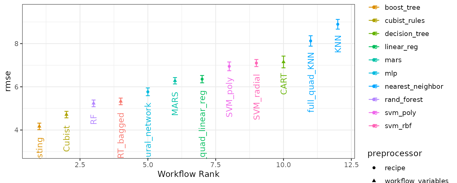
If you want to look at the tuning parameter results for a specific model:
autoplot(race_results, id = "neural_network", metric = "rmse") 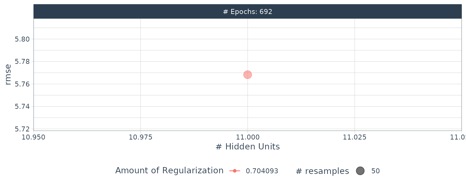
autoplot(race_results, id = "Cubist", metric = "rmse") 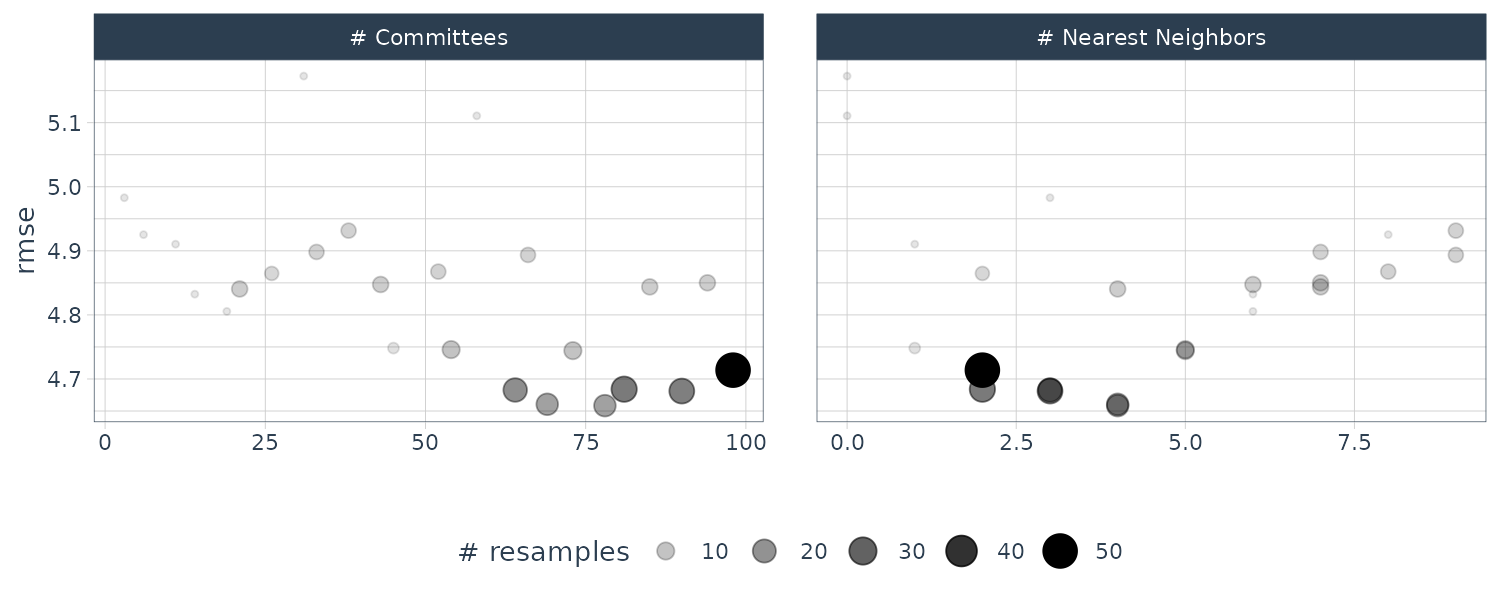
And performance metrics and prediction results:
> collect_metrics(race_results) |>
  select(-preproc)
# A tibble: 506 × 8
   wflow_id .config               model         .metric .estimator  mean     n std_err
   <chr>    <chr>                 <chr>         <chr>   <chr>      <dbl> <int>   <dbl>
 1 MARS     Preprocessor1_Model1  mars          rmse    standard   6.19      3 0.341
 2 MARS     Preprocessor1_Model1  mars          rsq     standard   0.855     3 0.0127
 3 MARS     Preprocessor1_Model2  mars          rmse    standard   6.28     50 0.0897
 4 MARS     Preprocessor1_Model2  mars          rsq     standard   0.855    50 0.00452
 5 CART     Preprocessor1_Model01 decision_tree rmse    standard   8.06      3 0.856
 6 CART     Preprocessor1_Model01 decision_tree rsq     standard   0.753     3 0.0433
 7 CART     Preprocessor1_Model02 decision_tree rmse    standard   7.43      4 0.413
 8 CART     Preprocessor1_Model02 decision_tree rsq     standard   0.801     4 0.00896
 9 CART     Preprocessor1_Model03 decision_tree rmse    standard   8.31      3 0.756
10 CART     Preprocessor1_Model03 decision_tree rsq     standard   0.737     3 0.0445
# ℹ 496 more rows
# ℹ Use `print(n = ...)` to see more rows

> collect_predictions(race_results)
# A tibble: 13,374 × 7
   wflow_id .config              preproc            model  .row compressive_strength .pred
   <chr>    <chr>                <chr>              <chr> <int>                <dbl> <dbl>
 1 MARS     Preprocessor1_Model2 workflow_variables mars      1                17.3  17.9
 2 MARS     Preprocessor1_Model2 workflow_variables mars      2                 2.33 -1.77
 3 MARS     Preprocessor1_Model2 workflow_variables mars      3                10.1   7.26
 4 MARS     Preprocessor1_Model2 workflow_variables mars      4                22.4  20.9
 5 MARS     Preprocessor1_Model2 workflow_variables mars      5                 3.32  1.53
 6 MARS     Preprocessor1_Model2 workflow_variables mars      6                 6.88  4.88
 7 MARS     Preprocessor1_Model2 workflow_variables mars      7                13.3  20.7
 8 MARS     Preprocessor1_Model2 workflow_variables mars      8                13.3  20.7
 9 MARS     Preprocessor1_Model2 workflow_variables mars      9                21.9  19.0
10 MARS     Preprocessor1_Model2 workflow_variables mars     10                18.2  25.6
# ℹ 13,364 more rows
# ℹ Use `print(n = ...)` to see more rows
Finalizing a Model
Manually picking “boosting” as the best result and finalizing workflow:
best_results <- race_results |>
  extract_workflow_set_result("boosting") |>
  select_best(metric = "rmse")

> best_results
# A tibble: 1 × 7
  trees min_n tree_depth learn_rate loss_reduction sample_size .config
  <int> <int>      <int>      <dbl>          <dbl>       <dbl> <chr>
1  1800    25          4      0.109       9.84e-10       0.850 Preprocessor1_Model16

boosting_test_results <- race_results |>
  extract_workflow("boosting") |>
  finalize_workflow(best_results) |>
  last_fit(split = concrete_split)

> boosting_test_results
# Resampling results
# Manual resampling
# A tibble: 1 × 6
  splits            id               .metrics         .notes           .predictions       .workflow
  <list>            <chr>            <list>           <list>           <list>             <list>
1 <split [743/249]> train/test split <tibble [2 × 4]> <tibble [0 × 3]> <tibble [249 × 4]> <workflow>
See the final test set results:
> collect_metrics(boosting_test_results)
# A tibble: 2 × 4
  .metric .estimator .estimate .config
  <chr>   <chr>          <dbl> <chr>
1 rmse    standard       3.52  Preprocessor1_Model1
2 rsq     standard       0.952 Preprocessor1_Model1
And visualizing the predictions:
boosting_test_results |>
  collect_predictions() |>
  ggplot(aes(x = compressive_strength, y = .pred)) +
  geom_abline(color = "gray50", lty = 2) +
  geom_point(alpha = 0.5) +
  coord_obs_pred() +
  labs(x = "observed", y = "predicted")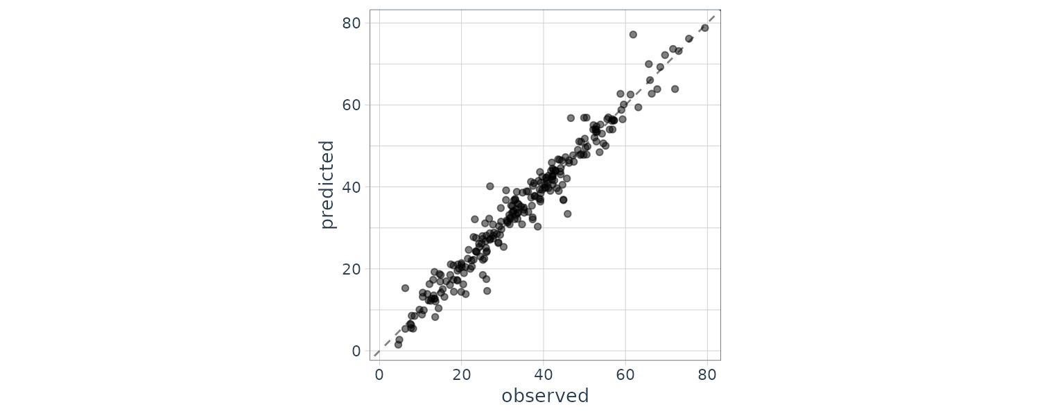
Dimensionality Reduction
Principal Component Analysis (PCA) is one of the most popular methdos for dimensionality reduction. For this section, we will use the beans dataset. Images of 13,611 grains of 7 different registered dry beans were taken with a high resolution camera.
The training data come from a set of manually labelled images. In the bean data, 16 morphology features were computed: area, perimeter, major axis length, minor axis length, aspect ratio, eccentricity, convex area, equivalent diameter, extent, solidity, roundness, compactness, shape factor1, shape factor 2, shape factor 3, and shape factor 4.
We will split the dataset into training and test set, and the validation sets:
bean_split <- initial_split(
  beans,
  strata = class,
  prop = 3 / 4
)

bean_train <- training(bean_split)
bean_test <- testing(bean_split)

bean_val <- validation_split(
  bean_train,
  strata = class,
  prop = 4 / 5
)
> bean_val
# Validation Set Split (0.8/0.2)  using stratification
# A tibble: 1 × 2
  splits              id
  <list>              <chr>
1 <split [8163/2043]> validation
> bean_val$splits[[1]]
<Training/Validation/Total>
<8163/2043/10206>
Many of the features have high correlations within themselves and we can see that by plotting the scatterplot matrix:
tmwr_cols <- colorRampPalette(c("#91CBD765", "#CA225E"))
bean_train |>
  dplyr::select(-class) |>
  cor() |>
  corrplot(
    col = tmwr_cols(200),
    tl.col = "black",
    method = "ellipse"
  )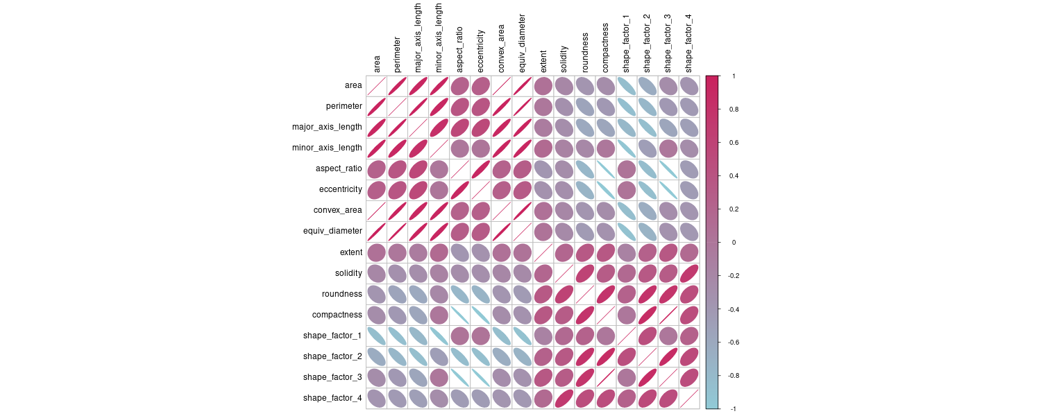
We can use step_orderNorm() in the bestNormalize package to enforce a symmetric distribution for the predictors. Also step_zv() remove variables that only contain a single value, and step_normalize() standardize variables to mean 0 and variance 1.
bean_rec <- recipe(
  class ~ .,
  data = analysis(bean_val$splits[[1]])
) |>
  step_zv(all_numeric_predictors()) |>
  step_orderNorm(all_numeric_predictors()) |>
  step_normalize(all_numeric_predictors())

> bean_rec
── Recipe ──────────────────────────────────────────────

── Inputs
Number of variables by role
outcome:    1
predictor: 16

── Operations
• Zero variance filter on: all_numeric_predictors()
• orderNorm transformation on: all_numeric_predictors()
• Centering and scaling for: all_numeric_predictors()
Preparing a Recipe
prep(recipe, training) fits the recipe to the training set, while bake(recipe, new_data) applies the recipe operations to new_data. For prep(), when retain=TRUE (by default), the pre-processed training data is saved within the recipe. For large training set, use retain=FALSE to avoid memory issue.
bean_rec_trained <- prep(bean_rec)

> bean_rec_trained
── Recipe ───────────────────────────────────────────────

── Inputs
Number of variables by role
outcome:    1
predictor: 16

── Operations
• Zero variance filter on: all_numeric_predictors()
• orderNorm transformation on: all_numeric_predictors()
• Centering and scaling for: all_numeric_predictors()
Baking the Recipe
Validation set samples can be assessed by:
bean_validation <- bean_val$splits |>
  pluck(1) |>
  assessment()
To process the validation set samples:
bean_val_processed <- bake(
  bean_rec_trained,
  new_data = bean_validation
)
Let us graph the histogram for the area predictor before and after processing:
library(patchwork)
p1 <- bean_validation |>
  ggplot(aes(x = area)) +
  geom_histogram(
    bins = 30,
    color = "white",
    fill = "blue",
    alpha = 1 / 3
  ) +
  ggtitle("Original validation set data")

p2 <- bean_val_processed |>
  ggplot(aes(x = area)) +
  geom_histogram(
    bins = 30,
    color = "white",
    fill = "red",
    alpha = 1 / 3
  ) +
  ggtitle("Processed validation set data")

p1 + p2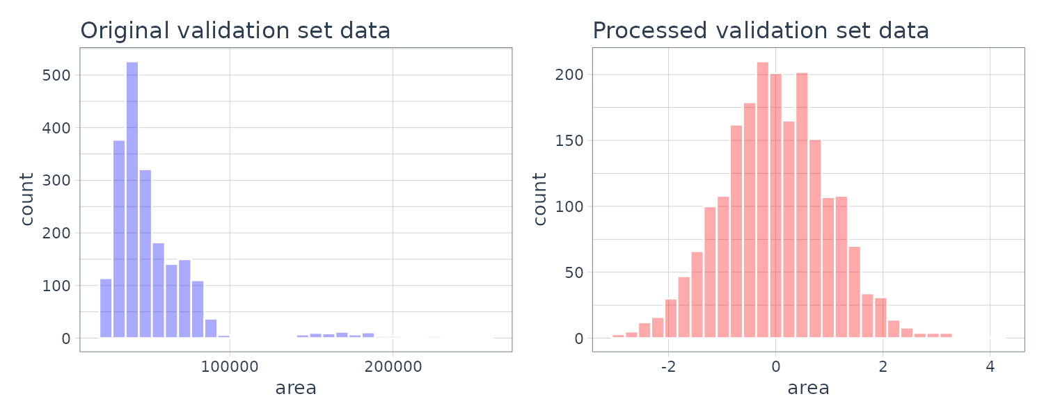
As for bake(), if retain=TRUE, we can get the prediction for training data using:
> bake(bean_rec_trained, new_data = NULL) |>
  nrow()
[1] 8163

> bean_val$splits |>
  pluck(1) |>
  analysis() |>
  nrow()
[1] 8163
We will create a helper function (for use later) to prep(), bake(), and plot the data:
plot_validation_results <- function(recipe, dat = assessment(bean_val$splits[[1]])) {
  set.seed(1)
  plot_data <- recipe |>
    prep() |>
    bake(new_data = dat, all_predictors(), all_outcomes()) |>
    sample_n(250)

  # Convert feature names to symbols to use with quasiquotation
  nms <- names(plot_data)
  x_name <- sym(nms[1])
  y_name <- sym(nms[2])

  plot_data |>
    ggplot(
      aes(
        x = !!x_name,
        y = !!y_name,
        col = class,
        fill = class,
        pch = class
      )
    ) +
    geom_point(alpha = 0.9) +
    scale_shape_manual(values = 1:7) +
    # Make equally sized axes
    coord_obs_pred() +
    theme_bw()
}
Principal Component Analysis (PCA)
PCA is an unsupervised method that uses linear combinations of the predictors to define new features which account for as much variation as possible. The number of components to retain as new predictors:
bean_rec_trained |>
  step_pca(
    all_numeric_predictors(),
    num_comp = 4
  ) |>
  plot_validation_results() +
ggtitle("Principal Component Analysis") 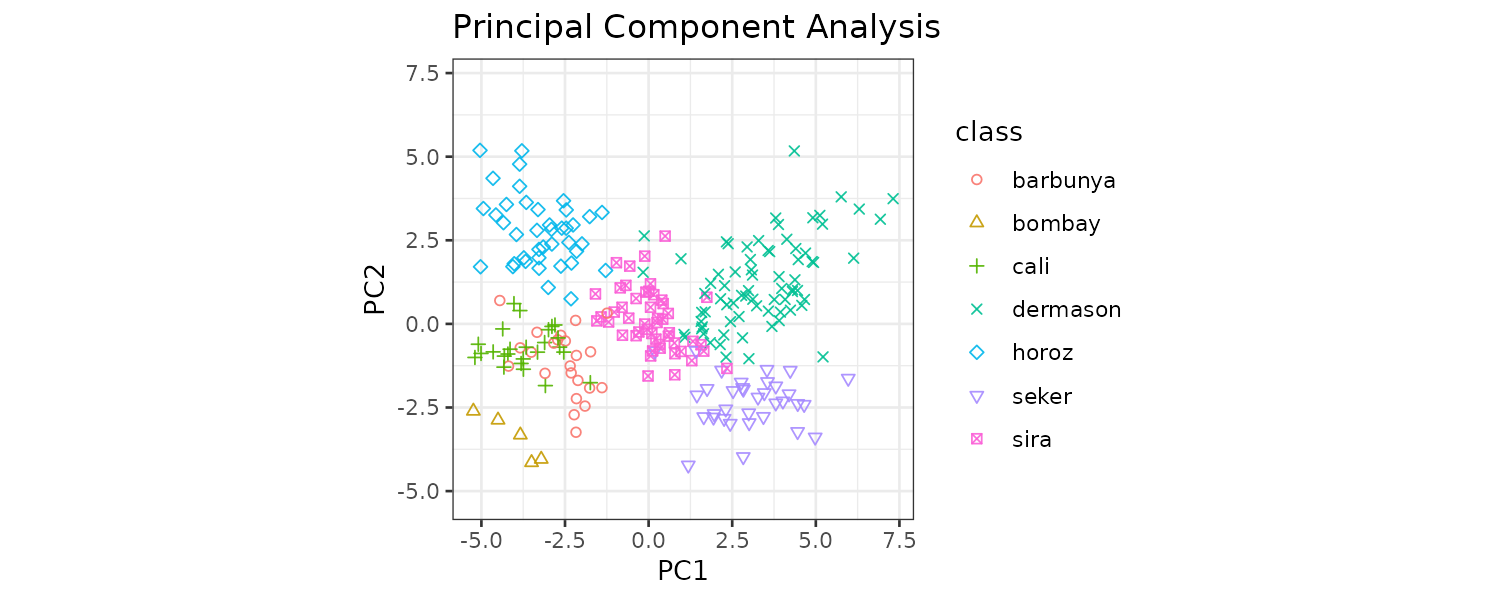
The “learntidymodels” package has functions that visualize the top features for each component:
library(learntidymodels)
bean_rec_trained |>
  step_pca(
    all_numeric_predictors(),
    num_comp = 4
  ) |>
  prep() |>
  plot_top_loadings(
    component_number <= 4,
    n = 5
  ) +
  scale_fill_brewer(palette = "Paired") +
ggtitle("Principal Component Analysis") 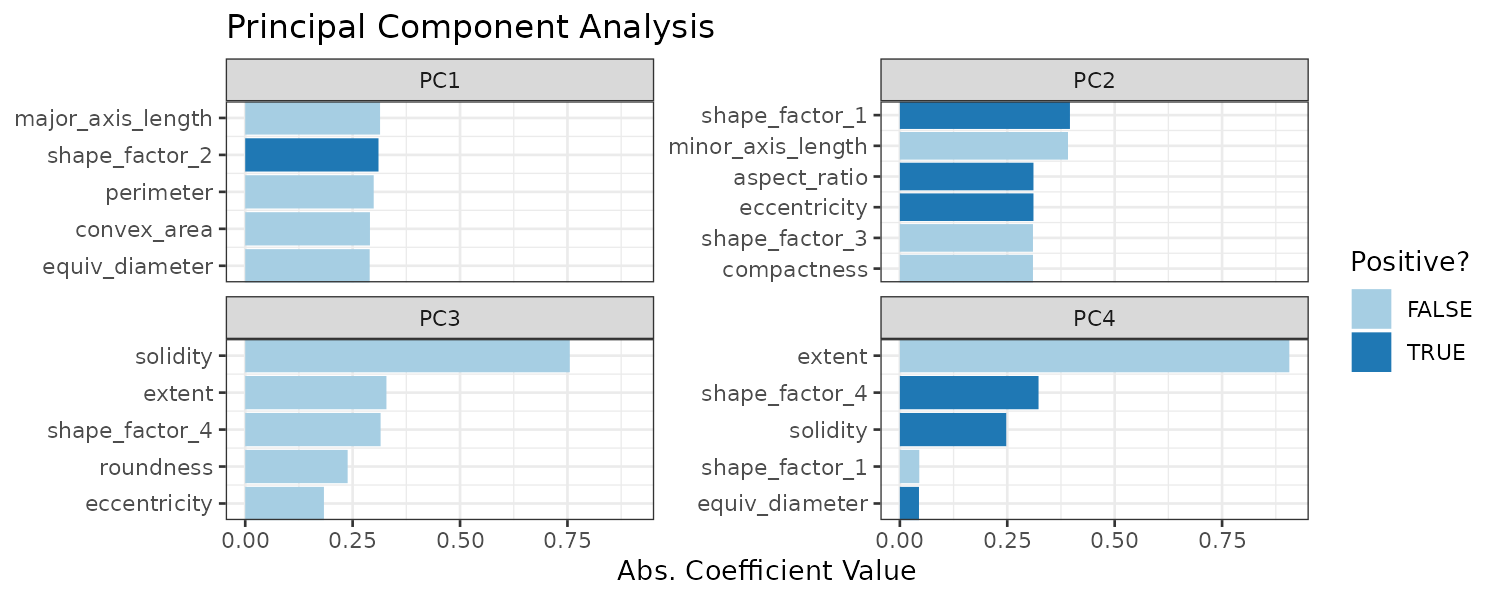
The top loadings are mostly related to size and the second loadings are related to measures of elongation.
Partial Least Squares (PLS)
PLS is a supervised version of PCA. On top of maximizing the variation in the predictors, it also maximize the relationship between the components and the outcome.
bean_rec_trained |>
  step_pls(
    all_numeric_predictors(),
    outcome = "class",
    num_comp = 4
  ) |>
  plot_validation_results() +
ggtitle("Partial Least Squares") 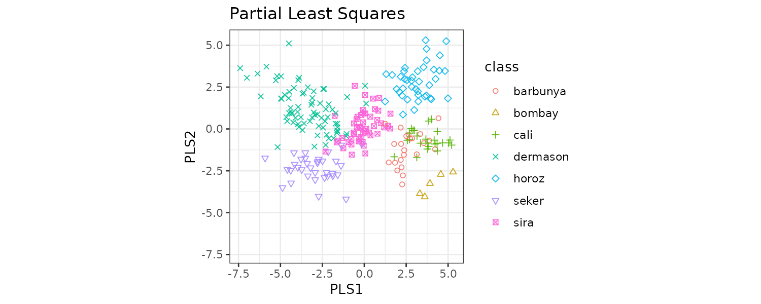
Looking at the top loadings:
bean_rec_trained |>
  step_pls(
    all_numeric_predictors(),
    outcome = "class",
    num_comp = 4
  ) |>
  prep() |>
  plot_top_loadings(
    component_number <= 4,
    n = 5,
    type = "pls"
  ) +
  scale_fill_brewer(palette = "Paired") +
  ggtitle("Partial Least Squares")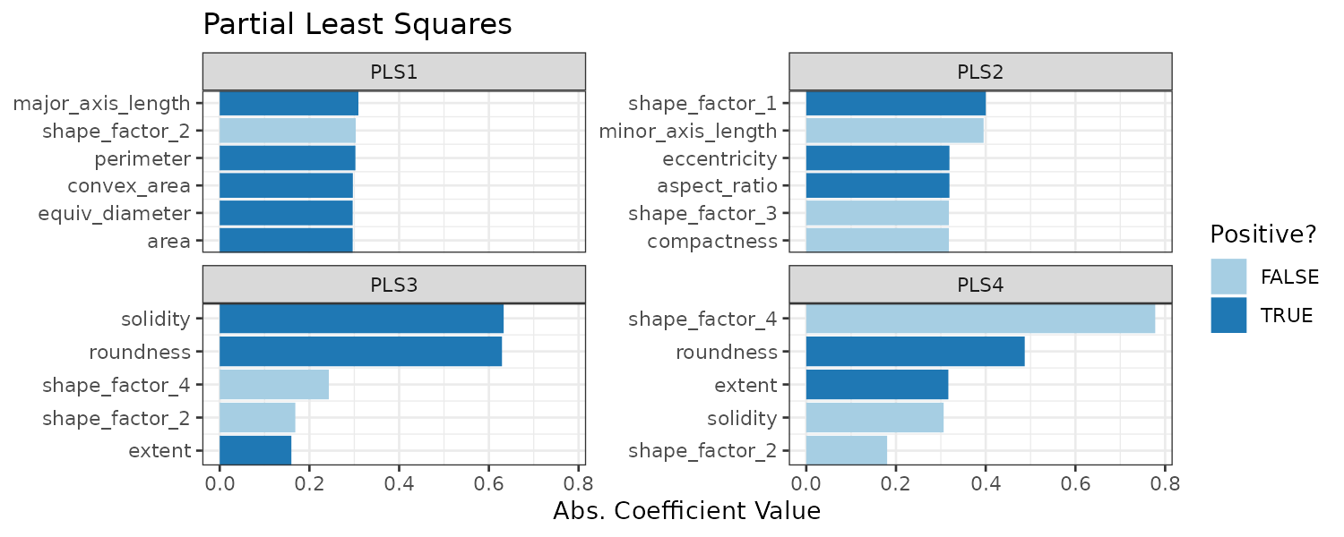
We can see the first two PLS components are similar to the first two PCA components. However the other components are different.
Independent Component Analysis (ICA)
ICA finds components that are as statistically independent from one another as possible. It can be thought of as maximizing the “Non-Gaussianity” of the ICA components. Rather than compressing information like PCA, it is trying to separate information.
bean_rec_trained |>
  step_ica(
    all_numeric_predictors(),
    num_comp = 4
  ) |>
  plot_validation_results() +
ggtitle("Independent Component Analysis") 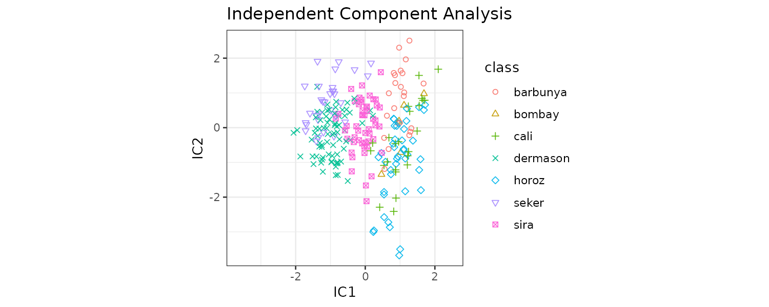
However, the ICA does not separate the bean classes well for the first 2 components.
Uniform Manifold Approximation and Projection (UMAP)
UMAP is similar to t-SNE method. UMAP uses Euclidean distance based on nearest neighbor method to find local areas where the data points are more likely to be related. The relationship between data points is saved as a directed graph model. To do this, the algorithm has an optimization process that uses cross-entropy to map data points to a smaller set of features.
library(embed)
bean_rec_trained |>
  step_umap(
    all_numeric_predictors(),
    num_comp = 4
  ) |>
  plot_validation_results() +
  ggtitle("UMAP")
There is also a supervised version of UMAP:
bean_rec_trained |>
  step_umap(
    all_numeric_predictors(),
    outcome = "class",
    num_comp = 4
  ) |>
  plot_validation_results() +
ggtitle("UMAP (supervised)") 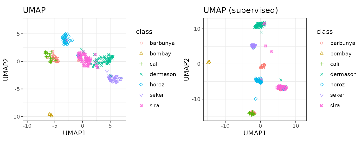
UMAP is a powerful method to reduce the feature space. However, it can be very sensitive to tuning parameters such as the number of neighbors, etc.
Modelling
Let’s explore models with dimensionality reduction added and along with no transformation at all. We would consider the following models:
- Naive Bayes
- Bagged Trees
- Single-Layer Neural Network
- Flexible Discriminant Analysis (FDA)
- Regularized Discriminant Analysis (RDA)
bayes_spec <- naive_Bayes() |>
  set_engine("klaR")

bagging_spec <- bag_tree() |>
  set_engine("rpart") |>
  set_mode("classification")

mlp_spec <- mlp(
  hidden_units = tune(),
  penalty = tune(),
  epochs = tune()
) |>
  set_engine("nnet") |>
  set_mode("classification")

fda_spec <- discrim_flexible(
    prod_degree = tune()
) |>
  set_engine("earth")

rda_spec <- discrim_regularized(
  frac_common_cov = tune(),
  frac_identity = tune()
) |>
  set_engine("klaR")
Next, we create recipe for PLS and UMAP sharing a common base recipe:
bean_rec <- recipe(class ~ ., data = bean_train) |>
  step_zv(all_numeric_predictors()) |>
  step_orderNorm(all_numeric_predictors()) |>
  step_normalize(all_numeric_predictors())

pls_rec <- bean_rec |>
  step_pls(
    all_numeric_predictors(),
    outcome = "class",
    num_comp = tune()
  )

umap_rec <- bean_rec |>
  step_umap(
    all_numeric_predictors(),
    outcome = "class",
    num_comp = tune(),
    neighbors = tune(),
    min_dist = tune()
  )
The workflow_set() takes the preprocessors and crosses them with the models. The workflow_map() applies grid search across 10 parameter combinations and the metric is area under the ROC curve:
ctrl <- control_grid(parallel_over = "everything")
bean_res <- workflow_set(
    preproc = list(
      basic = class ~ .,
      pls = pls_rec,
      umap = umap_rec
    ),
    models = list(
      bayes = bayes_spec,
      fda = fda_spec,
      rda = rda_spec,
      bag = bagging_spec,
      mlp = mlp_spec
    )
  ) |>
  workflow_map(
    verbose = TRUE,
    seed = 1603,
    resamples = bean_val,
    grid = 10,
    metrics = metric_set(roc_auc),
    control = ctrl
  )

> bean_res
# A workflow set/tibble: 15 × 4
   wflow_id    info             option    result
   <chr>       <list>           <list>    <list>
 1 basic_bayes <tibble [1 × 4]> <opts[4]> <rsmp[+]>
 2 basic_fda   <tibble [1 × 4]> <opts[4]> <tune[+]>
 3 basic_rda   <tibble [1 × 4]> <opts[4]> <tune[+]>
 4 basic_bag   <tibble [1 × 4]> <opts[4]> <rsmp[+]>
 5 basic_mlp   <tibble [1 × 4]> <opts[4]> <tune[+]>
 6 pls_bayes   <tibble [1 × 4]> <opts[4]> <tune[+]>
 7 pls_fda     <tibble [1 × 4]> <opts[4]> <tune[+]>
 8 pls_rda     <tibble [1 × 4]> <opts[4]> <tune[+]>
 9 pls_bag     <tibble [1 × 4]> <opts[4]> <tune[+]>
10 pls_mlp     <tibble [1 × 4]> <opts[4]> <tune[+]>
11 umap_bayes  <tibble [1 × 4]> <opts[4]> <tune[+]>
12 umap_fda    <tibble [1 × 4]> <opts[4]> <tune[+]>
13 umap_rda    <tibble [1 × 4]> <opts[4]> <tune[+]>
14 umap_bag    <tibble [1 × 4]> <opts[4]> <tune[+]>
15 umap_mlp    <tibble [1 × 4]> <opts[4]> <tune[+]>
Next we rank the models by their validation set based on the AUC:
rankings <- rank_results(
  bean_res,
  select_best = TRUE
) |>
  mutate(
    method = map_chr(
      wflow_id,
      ~ str_split(
        .x,
        "_",
        simplify = TRUE
      )[1]
    )
  )

> filter(rankings, rank <= 5) |>
  dplyr::select(
    rank,
    mean,
    model,
    method
  )
# A tibble: 5 × 4
   rank  mean model               method
  <int> <dbl> <chr>               <chr>
1     1 0.995 mlp                 pls
2     2 0.995 discrim_regularized pls
3     3 0.995 discrim_flexible    basic
4     4 0.994 naive_Bayes         pls
5     5 0.993 naive_Bayes         basic
We can plot the performance of various models:
rankings |>
  ggplot(
    aes(
      x = rank,
      y = mean,
      pch = method,
      color = model
    )
  ) +
  geom_point(cex = 3.5) +
  theme(legend.position = "right") +
  labs(y = "ROC AUC") +
  geom_text(
    aes(
      y = mean - 0.01,
      label = wflow_id
    ),
    angle = 90,
    hjust = 1
  ) +
  lims(y = c(0.9, NA))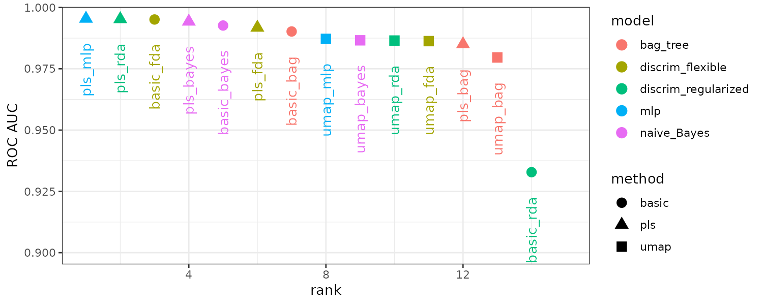
We will select the second best performing RDA model with PLS features as the final model. We will finalize the workflow with the best parameters, fit it with the training set, then evaluate with test set:
rda_res <- bean_res |>
  extract_workflow("pls_rda") |>
  finalize_workflow(
    bean_res |>
      extract_workflow_set_result("pls_rda") |>
      select_best(metric = "roc_auc")
  ) |>
  last_fit(
    split = bean_split,
    metrics = metric_set(roc_auc)
  )

> rda_res
# Resampling results
# Manual resampling
# A tibble: 1 × 6
  splits               id               .metrics         .notes           .predictions          .workflow
  <list>               <chr>            <list>           <list>           <list>                <list>
1 <split [10206/3405]> train/test split <tibble [1 × 4]> <tibble [0 × 3]> <tibble [3,405 × 10]> <workflow>
Extracting the actual fit:
rda_wflow_fit <- rda_res$.workflow[[1]]
> rda_wflow_fit
══ Workflow [trained] ═══════════════════════════════════════════════════════
Preprocessor: Recipe
Model: discrim_regularized()

── Preprocessor ─────────────────────────────────────────────────────────────
4 Recipe Steps

• step_zv()
• step_orderNorm()
• step_normalize()
• step_pls()

── Model ────────────────────────────────────────────────────────────────────
Call:
rda(formula = ..y ~ ., data = data, lambda = ~0.490939607401378,
    gamma = ~0.0270428076386452)

Regularization parameters:
     gamma     lambda
0.02704281 0.49093961

Prior probabilities of groups:
  barbunya     bombay       cali   dermason      horoz      seker       sira
0.09807956 0.03919263 0.11904762 0.25935724 0.14099549 0.14961787 0.19370958

Misclassification rate:
       apparent: 8.956 %
And the metrics:
> collect_metrics(rda_res)
# A tibble: 1 × 4
  .metric .estimator .estimate .config
  <chr>   <chr>          <dbl> <chr>
1 roc_auc hand_till      0.995 Preprocessor1_Model1
Encoding Categorical Data
Some models, such as those based on trees and rules, can handle categorical data natively and do not require encoding or transformation. Naive Bayes is another example that can deal with categorical variables natively.
Other models require the tranformation of categorical variable into a set of dummy or indicator variables. However, if there are too many categories or new cateogries at prediction, straighforward dummy variables are not a good fit.
For ordinal variables, in base R, the default encoding strategy is to make new numeric columns that are polynomial expansions of the data. For example, if there are 5 ordinal values, the factor column is relaced with 4 new columns, namely linear, quadratic, cubic, and quartic terms. However this form of encoding is not intuitive. Instead consider recipe steps related to order factors such as step_unorder() for regular factors and step_ordinalscore() for ordinal factors.
Effects Encoding
Effects encoding replaces categorical variables with a numeric column that measures the effect of the column. In the embed package, there are several recipe step functions for different kind of effect encodings:
- step_lencode_glm()
- step_lencode_mixed()
- step_lencode_bayes()
These steps use a generalized linear model to estimate the effect of each level.
For example, in the Ames housing data, we can compute the mean or median sale price for each neighborhood:
ames_train |>
  group_by(Neighborhood) |>
  summarize(
    mean = mean(Sale_Price),
    std_err = sd(Sale_Price) / sqrt(length(Sale_Price))
  ) |>
  ggplot(
    aes(
      y = reorder(Neighborhood, mean),
      x = mean
    )
  ) +
  geom_point() +
  geom_errorbar(
    aes(
      xmin = mean - 1.64 * std_err,
      xmax = mean + 1.64 * std_err
    )
  ) +
  labs(y = NULL, x = "Price (mean, log scale)") +
  theme_tq()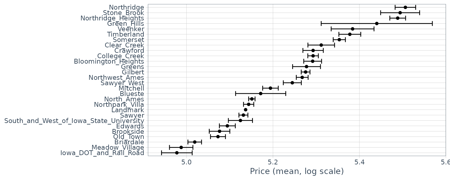
In this example, we use the step_lencode_glm() that replaces each categories with scores derived from a generalized linear model:
library(embed)
ames_glm <- recipe(
  Sale_Price ~ Neighborhood +
    Gr_Liv_Area +
    Year_Built +
    Bldg_Type +
    Latitude +
    Longitude,
  data = ames_train
) |>
  step_log(Gr_Liv_Area, base = 10) |>
  step_lencode_glm(Neighborhood, outcome = vars(Sale_Price)) |>
  step_dummy(all_nominal_predictors()) |>
  step_interact(~ Gr_Liv_Area:starts_with("Bldg_Type_")) |>
  step_ns(Latitude, Longitude, deg_free = 20)

> ames_glm
── Recipe ─────────────────────────────────────────────────

── Inputs
Number of variables by role
outcome:   1
predictor: 6

── Operations
• Log transformation on: Gr_Liv_Area
• Linear embedding for factors via GLM for: Neighborhood
• Dummy variables from: all_nominal_predictors()
• Interactions with: Gr_Liv_Area:starts_with("Bldg_Type_")
• Natural splines on: Latitude, Longitude
We can use tidy() to see the results of the scores. Number 2 refers to the glm step:
glm_estimates <- prep(ames_glm) |>
  tidy(number = 2)

> glm_estimates
# A tibble: 28 × 4
   level              value terms        id
   <chr>              <dbl> <chr>        <chr>
 1 North_Ames          5.15 Neighborhood lencode_glm_E0Wcj
 2 College_Creek       5.29 Neighborhood lencode_glm_E0Wcj
 3 Old_Town            5.06 Neighborhood lencode_glm_E0Wcj
 4 Edwards             5.10 Neighborhood lencode_glm_E0Wcj
 5 Somerset            5.35 Neighborhood lencode_glm_E0Wcj
 6 Northridge_Heights  5.49 Neighborhood lencode_glm_E0Wcj
 7 Gilbert             5.27 Neighborhood lencode_glm_E0Wcj
 8 Sawyer              5.13 Neighborhood lencode_glm_E0Wcj
 9 Northwest_Ames      5.27 Neighborhood lencode_glm_E0Wcj
10 Sawyer_West         5.25 Neighborhood lencode_glm_E0Wcj
# ℹ 18 more rows
# ℹ Use `print(n = ...)` to see more rows
Note that there is a level created for level not seen in the training data:
> glm_estimates |>
  filter(level == "..new")
# A tibble: 1 × 4
  level value terms        id
  <chr> <dbl> <chr>        <chr>
1 ..new  5.24 Neighborhood lencode_glm_E0Wcj
When you create an effect encoding for your categorical variable, you are effectively layering a mini-model inside your actual model which might result in overfitting.
Effect Encodings with Partial Pooling
Some factor level has very little samples so it make more sense to pool them together. The effects for each level are modeled all at once using a mixed or hierarchical generalized linear model:
ames_mixed <- recipe(
  Sale_Price ~ Neighborhood +
    Gr_Liv_Area +
    Year_Built +
    Bldg_Type +
    Latitude +
    Longitude,
  data = ames_train
) |>
  step_log(Gr_Liv_Area, base = 10) |>
  step_lencode_mixed(
    Neighborhood,
    outcome = vars(Sale_Price)
  ) |>
  step_dummy(all_nominal_predictors()) |>
  step_interact(~ Gr_Liv_Area:starts_with("Bldg_Type_")) |>
  step_ns(Latitude, Longitude, deg_free = 20)

> ames_mixed
── Recipe ─────────────────────────────────────────────────────────

── Inputs
Number of variables by role
outcome:   1
predictor: 6

── Operations
• Log transformation on: Gr_Liv_Area
• Linear embedding for factors via mixed effects for: Neighborhood
• Dummy variables from: all_nominal_predictors()
• Interactions with: Gr_Liv_Area:starts_with("Bldg_Type_")
• Natural splines on: Latitude, Longitude
As we can see the number of levels is less:
mixed_estimates <- prep(ames_mixed) |>
  tidy(number = 2)

> mixed_estimates
# A tibble: 29 × 4
   level              value terms        id
   <chr>              <dbl> <chr>        <chr>
 1 North_Ames          5.16 Neighborhood lencode_mixed_Ljmpx
 2 College_Creek       5.29 Neighborhood lencode_mixed_Ljmpx
 3 Old_Town            5.07 Neighborhood lencode_mixed_Ljmpx
 4 Edwards             5.09 Neighborhood lencode_mixed_Ljmpx
 5 Somerset            5.35 Neighborhood lencode_mixed_Ljmpx
 6 Northridge_Heights  5.50 Neighborhood lencode_mixed_Ljmpx
 7 Gilbert             5.28 Neighborhood lencode_mixed_Ljmpx
 8 Sawyer              5.13 Neighborhood lencode_mixed_Ljmpx
 9 Northwest_Ames      5.26 Neighborhood lencode_mixed_Ljmpx
10 Sawyer_West         5.25 Neighborhood lencode_mixed_Ljmpx
# ℹ 19 more rows
# ℹ Use `print(n = ...)` to see more rows
The neighborhoods with the fewest homes in them have been pulled (either up or down) toward the mean effect. When we use pooling, we shrink the effect estimates toward the mean because we don’t have as much evidence about the price in those neighborhoods.
Explaining Models
For certain models, it is easier to explain why the model makes its predictions. For example, linear regression contains coefficients for each predictor that are easy to interpret. For models like random forest, it is less clear. But with the help of DALEX package, we can apply model explainer algorithms to help understanding.
Models trained with tidymodels have to explained with other supplementary software in R packages such as lime, vip, and DALEX.
vip functions use model-based methods that take advantage of model structure and generally faster.
DALEX functions use model-agnostic methods that can be applied to any model.
Local Explanations
To start, we use a simple linear regression model to showcase the functionality of DALEX:
library(DALEXtra)

vip_features <- c(
  "Latitude",
  "Longitude"
)

vip_train <- ames_train |>
  select(all_of(vip_features))

simple_ames <- recipe(
  Sale_Price ~ Longitude + Latitude,
  data = ames_train
) |>
  step_normalize(all_numeric_predictors())
simple_ames

lm_wflow <- workflow() |>
  add_model(
    linear_reg() |>
      set_engine("lm")
  ) |>
  add_recipe(simple_ames)
lm_wflow

lm_fit <- fit(lm_wflow, ames_train)
We then create an explainer in R for the lm model:
explainer_lm <- explain_tidymodels(
    lm_fit,
    data = vip_train,
    y = ames_train$Sale_Price,
    label = "lm",
    verbose = FALSE
  )

fit <- lm_fit |>
  extract_fit_parsnip()

> fit
parsnip model object


Call:
stats::lm(formula = ..y ~ ., data = data)

Coefficients:
(Intercept)    Longitude     Latitude
    5.22031     -0.05328      0.05302
Taking an example from training data:
duplex <- vip_train[120, ]

> duplex
# A tibble: 1 × 2
  Latitude Longitude
     <dbl>     <dbl>
1     42.0     -93.6
And attempting to explain by DALEX function predict_parts():
lm_breakdown <- predict_parts(
explainer = explainer_lm,
new_observation = duplex
)
> lm_breakdown
contribution
lm: intercept 5.220
lm: Longitude = -93.614049 -0.060
lm: Latitude = 42.036015 0.004
lm: prediction 5.165We can see that the contribution column is similar but not exact to the coefficients from lm. Let’s check the prediction from the fit:
> predict(lm_fit, duplex)
# A tibble: 1 × 1
.pred
<dbl>
1 5.17We can see the prediction is exactly the same as the explain model. I reckon some of the explaination is shifted to Longitude from Latitude.
Now let’s expand the predictors which include interactions and splines:
simple_ames <- recipe(
Sale_Price ~ Neighborhood +
Gr_Liv_Area +
Year_Built +
Bldg_Type +
Latitude,
data = ames_train
) |>
step_log(Gr_Liv_Area, base = 10) |>
step_other(Neighborhood, threshold = 0.01) |>
step_dummy(all_nominal_predictors()) |>
step_interact(~ Gr_Liv_Area:starts_with("Bldg_Type_")) |>
step_ns(Latitude, deg_free = 20)
> lm_breakdown
contribution
lm + interactions: intercept 5.219
lm + interactions: Gr_Liv_Area = 1133 -0.061
lm + interactions: Year_Built = 1950 -0.043
lm + interactions: Neighborhood = 1 -0.030
lm + interactions: Bldg_Type = 1 0.009
lm + interactions: Latitude = 42.035787 0.005
lm + interactions: Longitude = -93.61061 0.000
lm + interactions: prediction 5.099 Because this linear model is trained with spline terms for Latitude and Longitude, the contributions combines the effects of the spline terms.
Let’s fit another random forest model:
rf_wflow <- workflow() |>
add_model(
rand_forest(trees = 1000, min_n = 5) |>
set_engine("ranger") |>
set_mode("regression")
) |>
add_recipe(simple_ames)
rf_fit <- fit(rf_wflow, ames_train)
explainer_rf <- explain_tidymodels(
rf_fit,
data = vip_train,
y = ames_train$Sale_Price,
label = "random forest",
verbose = FALSE
)
rf_breakdown <- predict_parts(
explainer = explainer_rf,
new_observation = duplex
)
> rf_breakdown
contribution
random forest: intercept 5.219
random forest: Gr_Liv_Area = 1133 -0.048
random forest: Latitude = 42.035787 -0.032
random forest: Year_Built = 1950 -0.046
random forest: Bldg_Type = 1 0.003
random forest: Neighborhood = 1 -0.002
random forest: Longitude = -93.61061 0.000
random forest: prediction 5.093 Notice that the importance ranking is different for random forest and linear regression.
If we choose the order for the random forest model explanation to be the same as the default for the linear model (chosen via a heuristic), we can change the relative importance of the features.
> predict_parts(
explainer = explainer_rf,
new_observation = duplex,
order = lm_breakdown$variable_name
)
contribution
random forest: intercept 5.221
random forest: Bldg_Type = 3 -0.025
random forest: Gr_Liv_Area = 1040 -0.045
random forest: Year_Built = 1949 -0.059
random forest: Neighborhood = 1 -0.012
random forest: Latitude = 42.035841 -0.085
random forest: Longitude = -93.608903 0.000
random forest: prediction 4.995 Because the explanations change based on order, we can use Shapley additive explanations (SHAP), where the average contributions of features are computed under different combinations of feature orderings. Let’s compute SHAP attributions for our duplex using B = 20 random orderings:
set.seed(1801)
shap_duplex <- predict_parts(
explainer = explainer_rf,
new_observation = duplex,
type = "shap",
B = 20
)
min q1 median mean q3 max
random forest: Bldg_Type = Duplex -0.07029846 -0.070298465 -0.028983381 -0.039620833 -0.024709960 -0.0130451793
random forest: Gr_Liv_Area = 1040 -0.07135597 -0.057113155 -0.053390380 -0.053390380 -0.045920685 -0.0442282141
random forest: Latitude = 42.04 -0.08451533 -0.067121217 -0.055863581 -0.060015024 -0.048660201 -0.0363856489
random forest: Longitude = -93.61 0.00000000 0.000000000 0.000000000 0.000000000 0.000000000 0.0000000000
random forest: Neighborhood = North_Ames -0.01389459 -0.008252223 -0.004621661 -0.006000526 -0.002838158 -0.0005413983
random forest: Year_Built = 1949 -0.08952797 -0.089527965 -0.059622599 -0.067231263 -0.058449223 -0.0508630795 We can plot this result in R. The box plots display the distribution of contributions across all the orderings we tried, and the bars display the average attribution for each feature:
library(forcats)
shap_duplex |>
group_by(variable) |>
mutate(
mean_val = mean(contribution)
) |>
ungroup() |>
mutate(
variable = fct_reorder(variable, abs(mean_val))
) |>
ggplot(
aes(
contribution,
variable,
fill = mean_val > 0
)
) +
geom_col(
data = ~ distinct(., variable, mean_val),
aes(mean_val, variable),
alpha = 0.5
) +
geom_boxplot(width = 0.5) +
theme_tq() +
theme(legend.position = "none") +
scale_fill_viridis_d() +
labs(y = NULL)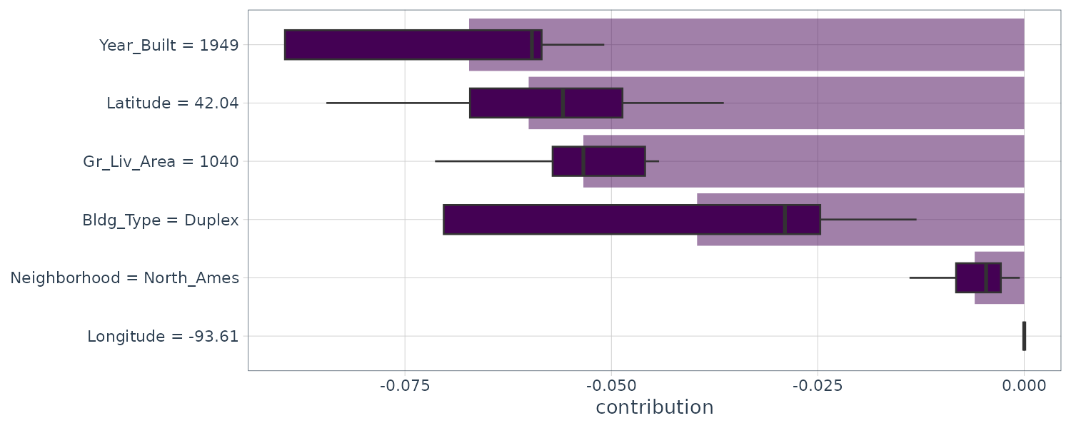
Global Explanations
Previously we addressed which variables are most important in predicting sale price for a single home. Global feature importance however addresses the most important variables for a model in aggregate.
One way to calculate this is to shuffle/permute the features to measure how much worse the model fits the data compared to before shuffling.
In DALE, we can compute this kind of variable importance via model_parts():
set.seed(1803)
vip_lm <- model_parts(
explainer_lm,
loss_function = loss_root_mean_square
)
> vip_lm
variable mean_dropout_loss label
1 _full_model_ 0.07650906 lm + interactions
2 Longitude 0.07650906 lm + interactions
3 Bldg_Type 0.08755229 lm + interactions
4 Latitude 0.09931083 lm + interactions
5 Year_Built 0.11710960 lm + interactions
6 Neighborhood 0.12570252 lm + interactions
7 Gr_Liv_Area 0.14252756 lm + interactions
8 _baseline_ 0.23096000 lm + interactions In this example, Gr_Liv_Area has the most importance because dropping it result in the largest increase in RMSE.
Building Global Explanations from Local Explanations
Previously we touched on local explanations for a single observation (via Shapley additive explanations) and also global model explanations for the whole dataset by permuting features. It is also possible to build a global model explanations by aggregating local model explanations. Partial dependence profiles show how the expected value of a model prediction, changes as a function of a feature.
One way is to build a profile by aggregating or averaging profiles for individual observations. A Ceteris Paribus (CP) profile shows how an individual observation prediction changes as a function of a given feature. We can employ DALEX model_profile() to accomplish this:
set.seed(1805)
pdp_age <- model_profile(
explainer_rf,
N = 500,
variables = "Year_Built"
)
> pdp_age
Top profiles :
_vname_ _label_ _x_ _yhat_ _ids_
1 Year_Built random forest 1872 5.166747 0
2 Year_Built random forest 1875 5.166747 0
3 Year_Built random forest 1880 5.166881 0
4 Year_Built random forest 1882 5.166890 0
5 Year_Built random forest 1885 5.166563 0
6 Year_Built random forest 1890 5.166226 0 The profiles are grouped by “ids” and we can graph each and also aggregate a mean profile:
ggplot_pdp <- function(obj, x) {
p <- as_tibble(obj$agr_profiles) |>
mutate(
`_label_` =
stringr::str_remove(`_label_`, "^[^_]*_")) |>
ggplot(aes(`_x_`, `_yhat_`)) +
geom_line(
data = as_tibble(obj$cp_profiles),
aes(x = , group = `_ids_`),
size = 0.5,
alpha = 0.05,
color = "gray50"
)
num_colors <- n_distinct(obj$agr_profiles$`_label_`)
if (num_colors > 1) {
p <- p +
geom_line(
aes(color = `_label_`, lty = `_label_`),
size = 1.2
)
} else {
p <- p +
geom_line(
color = "midnightblue",
size = 1.2,
alpha = 0.8
)
}
p
}
ggplot_pdp(pdp_age, Year_Built) +
labs(
x = "Year built",
y = "Sale Price (log)",
color = NULL
) +
theme_tq()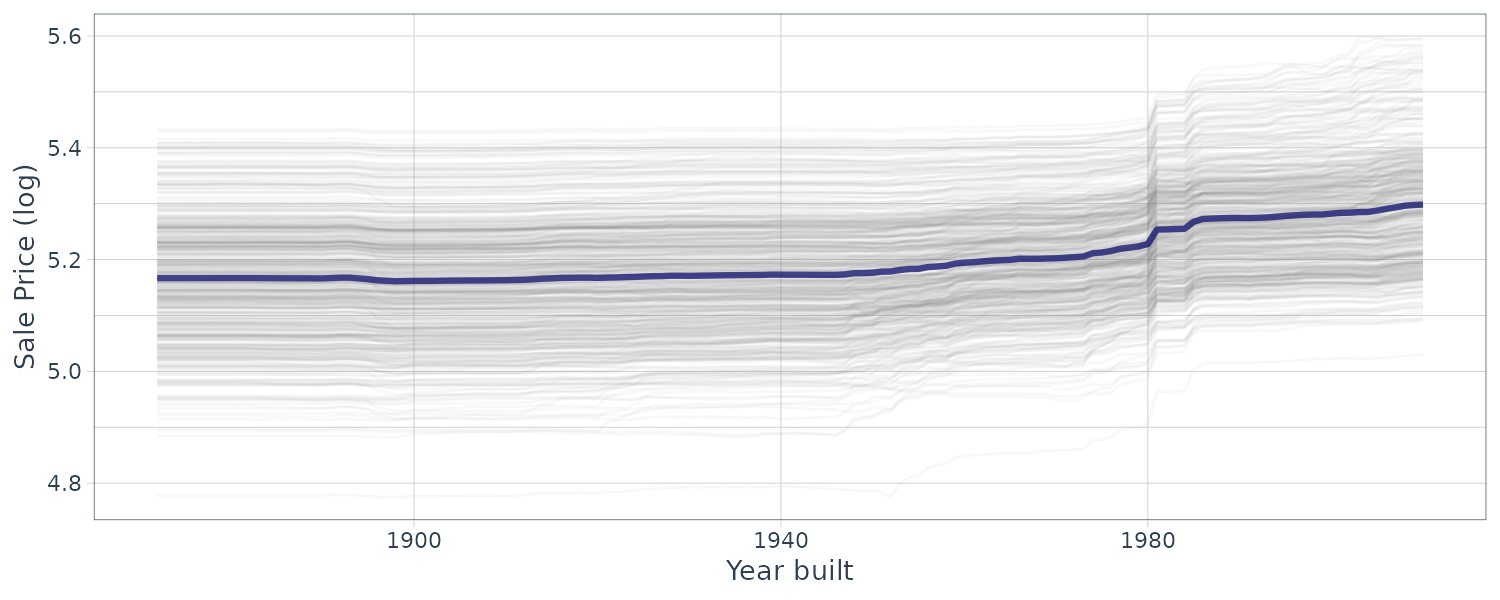
Prediction Quality
A predictive model can almost always produce a prediction. When a new data point is well outside of the range of data used to create the model, causing inappropriate extrapolation.
There are two methods for quantifying potential prediction quality:
- Equivocal Zones
- Applicability
Equivocal Results
Equivocal zone is a range of results in which the prediction should not be reported as positive as the prediction is too uncertain.
Suppose we have the following true logistic model:
\[\begin{aligned} \text{logit}(p) &= -1 - 2x - \frac{x^{2}}{5} + 2y^{2} \end{aligned}\]Both parameters are bivariate normal distributions with a correlation of 0.70. We create a training set of 200 samples and test set of 50 samples:
simulate_two_classes <-
function(n,
error = 0.1,
eqn = quote(-1 - 2 * x - 0.2 * x^2 + 2 * y^2)) {
# Slightly correlated predictors
sigma <- matrix(
c(1, 0.7, 0.7, 1),
nrow = 2,
ncol = 2
)
dat <- MASS::mvrnorm(
n = n,
mu = c(0, 0),
Sigma = sigma
)
colnames(dat) <- c("x", "y")
cls <- paste0("class_", 1:2)
dat <- as_tibble(dat) |>
mutate(
linear_pred = !!eqn,
# Add some misclassification noise
linear_pred = linear_pred + rnorm(n, sd = error),
prob = binomial()$linkinv(linear_pred),
class = ifelse(prob > runif(n), cls[1], cls[2]),
class = factor(class, levels = cls)
)
select(dat, x, y, class)
}
set.seed(1901)
training_set <- simulate_two_classes(200)
testing_set <- simulate_two_classes(50)
> testing_set
# A tibble: 50 × 3
x y class
<dbl> <dbl> <fct>
1 1.12 -0.176 class_2
2 -0.126 -0.582 class_2
3 1.92 0.615 class_2
4 -0.400 0.252 class_2
5 1.30 1.09 class_1
6 2.59 1.36 class_2
7 -0.610 0.123 class_2
8 -0.569 0.512 class_1
9 1.28 0.134 class_2
10 -0.408 -0.368 class_2
# ℹ 40 more rows
# ℹ Use `print(n = ...)` to see more rowsWe estimate a logistic regression model using Bayesian methods, using Gaussian as prior distributions:
two_class_mod <- logistic_reg() |>
set_engine("stan", seed = 1902) |>
fit(
class ~ . + I(x^2) + I(y^2),
data = training_set
)
> print(two_class_mod, digits = 3)
parsnip model object
stan_glm
family: binomial [logit]
formula: class ~ . + I(x^2) + I(y^2)
observations: 200
predictors: 5
------
Median MAD_SD
(Intercept) 1.092 0.287
x 2.290 0.423
y 0.314 0.354
I(x^2) 0.077 0.307
I(y^2) -2.465 0.424
------
* For help interpreting the printed output see ?print.stanreg
* For info on the priors used see ?prior_summary.stanregPreparing the prediction data:
data_grid <- crossing(
x = seq(-4.5, 4.5, length = 100),
y = seq(-4.5, 4.5, length = 100)
)
grid_pred <- predict(
two_class_mod,
data_grid,
type = "prob"
) |>
bind_cols(
predict(
two_class_mod,
data_grid,
type = "pred_int",
std_error = TRUE
),
data_grid
)Graphing the data:
grid_pred |>
mutate(
`Probability of Class 1` = .pred_class_1
) |>
ggplot(aes(x = x, y = y)) +
geom_raster(aes(fill = `Probability of Class 1`)) +
geom_point(
data = testing_set,
aes(
shape = class,
color = class),
alpha = .75,
size = 2.5
) +
geom_contour(
aes(z = .pred_class_1),
breaks = .5,
color = "black",
lty = 2
) +
coord_equal() +
labs(
x = "Predictor x",
y = "Predictor y",
color = NULL,
shape = NULL
) +
scale_fill_gradient2(
low = "#FDB863",
mid = "white",
high = "#B2ABD2",
midpoint = .5
) +
scale_color_manual(
values = c("#2D004B", "darkorange")
) +
theme_tq()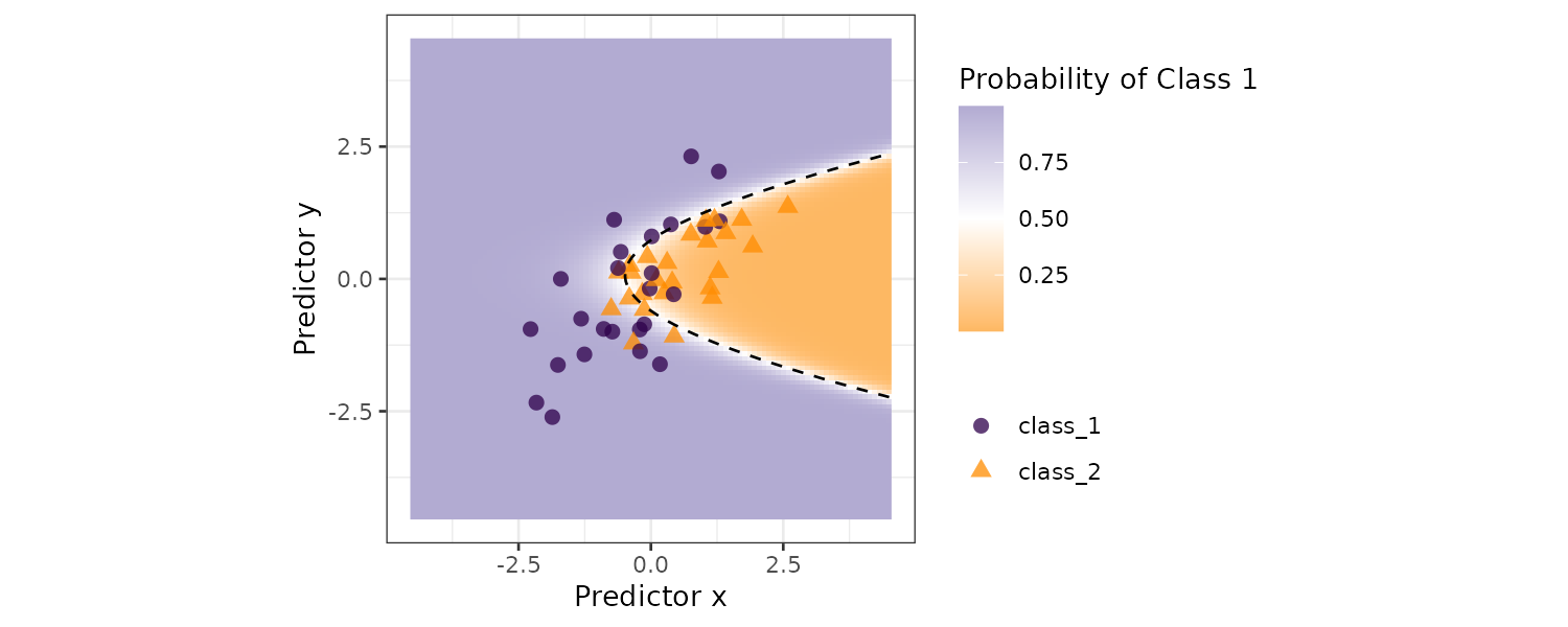
The “probably” package contains functions for equivocal zones. Rows that are within \(0.50 \pm 0.15\) are given a value of [EQ]:
library(probably)
lvls <- levels(training_set$class)
test_pred <- test_pred |>
mutate(
.pred_with_eqz = make_two_class_pred(
.pred_class_1,
lvls,
buffer = 0.15
)
)
> test_pred |>
count(.pred_with_eqz)
# A tibble: 3 × 2
.pred_with_eqz n
<clss_prd> <int>
1 [EQ] 9
2 class_1 20
3 class_2 21Contrasting the two confusion matrices:
> test_pred |>
conf_mat(class, .pred_class)
Truth
Prediction class_1 class_2
class_1 20 6
class_2 5 19
> test_pred |>
conf_mat(class, .pred_with_eqz)
Truth
Prediction class_1 class_2
class_1 17 3
class_2 5 16Rather than using predicted class probability to disqualify data points, a slightly better approach is to use the standard error of the class probability. One important aspect of the standard error is that it will increase where there is significant extrapolation. The Bayesian model naturally estimates the standard error of prediction.
grid_pred |>
mutate(
`Std Error` = .std_error
) |>
ggplot(
aes(x = x, y = y)
) +
geom_raster(
aes(fill = `Std Error`)
) +
scale_fill_gradient(
colours = c(
"#F7FBFF",
"#DEEBF7",
"#C6DBEF",
"#9ECAE1",
"#6BAED6")
) +
geom_point(
data = testing_set,
aes(shape = class),
alpha = .5,
size = 2
) +
coord_equal() +
labs(
x = "Predictor x",
y = "Predictor y",
shape = NULL
) +
theme_bw()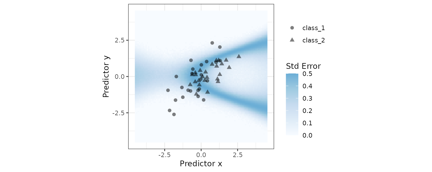
Applicability
Equivocal zones try to measure the reliability of a prediction based on the model outputs. However, model statistics such a she standard error of prediction might not be able to measure the impact of extrapolation.
Taking the example of ridership in Chicago. We can see that the model performs really badly from the 2020 data due to Covid in the book. Over here, we will use PCA to see if the test data is very far from the training data by computing scores along with the distnace to the center of the training set.
The applicable package can develop an applicability domain model using PCA. We indicate a threshold of 99%, such that the number of predictors are retained to ensure the treshold is maintained.
library(applicable)
pca_stat <- apd_pca(
~.,
data = Chicago_train |>
select(one_of(stations)),
threshold = 0.99
)
> pca_stat
# Predictors:
20
# Principal Components:
9 components were needed
to capture at least 99% of the
total variation in the predictors. Plotting the percentile of data points distance from the center of training data:
autoplot(pca_stat, distance) +
labs(x = "distance")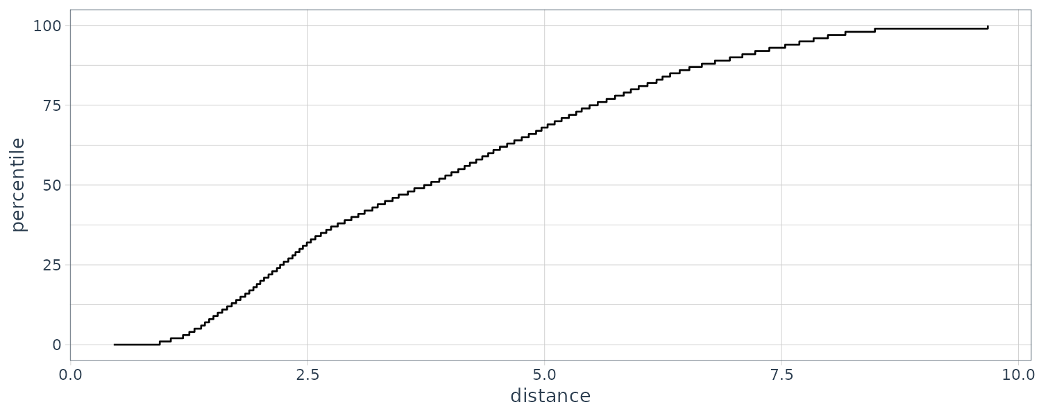
Computing the distance score and percentile for test data:
> score(pca_stat, Chicago_test) |>
select(starts_with("distance"))
# A tibble: 14 × 2
distance distance_pctl
<dbl> <dbl>
1 4.88 66.7
2 5.21 71.4
3 5.19 71.1
4 5.00 68.5
5 4.36 59.3
6 4.10 55.2
7 5.59 76.4
8 4.21 56.9
9 4.94 67.5
10 4.93 67.4
11 4.93 67.3
12 3.50 47.4
13 3.89 52.1
14 5.42 74.4And computing for 2020 data:
> score(pca_stat, Chicago_2020) |>
select(starts_with("distance"))
# A tibble: 14 × 2
distance distance_pctl
<dbl> <dbl>
1 9.39 99.8
2 9.40 99.8
3 9.30 99.7
4 9.30 99.7
5 9.29 99.7
6 10.1 1
7 10.2 1
8 10.1 1
9 9.30 99.7
10 9.22 99.6
11 9.26 99.7
12 9.12 99.5
13 9.80 1
14 10.7 1 We can clearly see that the 2020 data is way off the center.
Ensembles of Models
A model ensemble is the aggregation of predictions of multiple single learners. In this section, we will talk about aggregating different type of models known as model stacking.
A stacking model can include different types of models (e.g. trees and neural networks) and different configurations of the same model (e.g. trees with different depths).
We will use the race_results workflow set that we created earlier on:
> race_results
# A workflow set/tibble: 12 × 4
wflow_id info option result
<chr> <list> <list> <list>
1 MARS <tibble [1 × 4]> <opts[3]> <race[+]>
2 CART <tibble [1 × 4]> <opts[3]> <race[+]>
3 CART_bagged <tibble [1 × 4]> <opts[3]> <rsmp[+]>
4 RF <tibble [1 × 4]> <opts[3]> <race[+]>
5 boosting <tibble [1 × 4]> <opts[3]> <race[+]>
6 Cubist <tibble [1 × 4]> <opts[3]> <race[+]>
7 SVM_radial <tibble [1 × 4]> <opts[3]> <race[+]>
8 SVM_poly <tibble [1 × 4]> <opts[3]> <race[+]>
9 KNN <tibble [1 × 4]> <opts[3]> <race[+]>
10 neural_network <tibble [1 × 4]> <opts[4]> <race[+]>
11 full_quad_linear_reg <tibble [1 × 4]> <opts[3]> <race[+]>
12 full_quad_KNN <tibble [1 × 4]> <opts[3]> <race[+]> Next, we create an empty data stack and add candidate models:
concrete_stack <- stacks() |>
add_candidates(race_results)
> concrete_stack
# A data stack with 12 model definitions and 18 candidate members:
# MARS: 1 model configuration
# CART: 1 model configuration
# CART_bagged: 1 model configuration
# RF: 1 model configuration
# boosting: 1 model configuration
# Cubist: 1 model configuration
# SVM_radial: 1 model configuration
# SVM_poly: 1 model configuration
# KNN: 3 model configurations
# neural_network: 1 model configuration
# full_quad_linear_reg: 5 model configurations
# full_quad_KNN: 1 model configuration
# Outcome: compressive_strength (numeric)Meta-Learning Model
The different models are combined into a meta-learning model. Any model can be used but the most commonly used model is a regularized GLM which includes linear, logistc, and multinomial models. Specifically, regularization via the lasso penalty can help to reduce the number of candidates and also alleviate ehe problem of high correlation between ensemble candidates. By default, the blending coefficients are nonnegative but can be changed via an optional argument.
Because the outcome is numeric, linear regression is used for the metamodel:
set.seed(2001)
ens <- blend_predictions(concrete_stack)
> ens
── A stacked ensemble model ─────────────────────────────────
Out of 18 possible candidate members, the ensemble retained 7.
Penalty: 0.01.
Mixture: 1.
The 7 highest weighted members are:
# A tibble: 7 × 3
member type weight
<chr> <chr> <dbl>
1 boosting_1_16 boost_tree 0.744
2 Cubist_1_25 cubist_rules 0.156
3 full_quad_linear_reg_1_16 linear_reg 0.0348
4 neural_network_1_16 mlp 0.0336
5 CART_1_05 decision_tree 0.0206
6 full_quad_linear_reg_1_17 linear_reg 0.0182
7 MARS_1_2 mars 0.00988
Members have not yet been fitted with `fit_members()`.Plotting the performance metrics with the default penalization:
autoplot(ens) 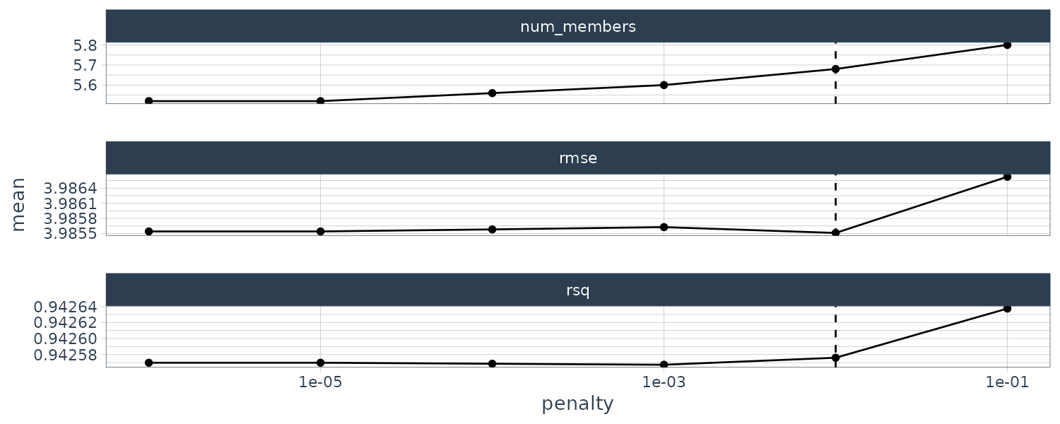
We can increase the penalty by passing down the parameter:
set.seed(2002)
ens <- blend_predictions(
concrete_stack,
penalty = 10^seq(-2, -0.5, length = 20)
)And plotting the performance metrics again with the new penalization range:
autoplot(ens) 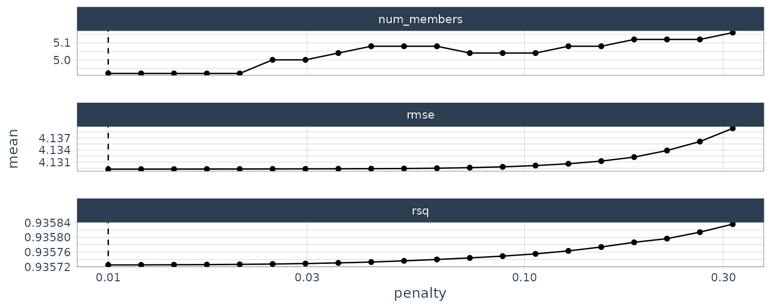
Let’s plot the contribution of each model type:
autoplot(ens, "weights") +
geom_text(
aes(x = weight + 0.01, label = model),
hjust = 0
) +
theme(legend.position = "none") +
lims(x = c(-0.01, 0.8)) +
theme_tq()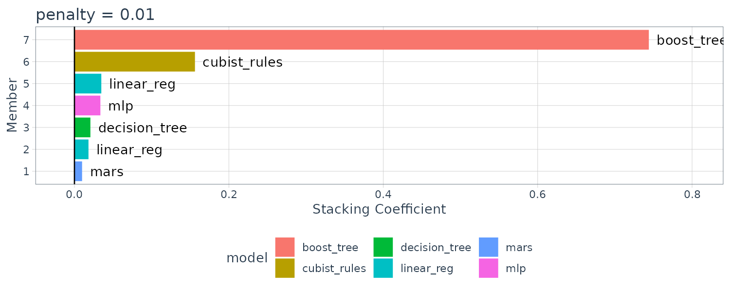
To be able to use the stacking model for prediction, we first need to fit the stacking model:
library(rules)
ens <- fit_members(ens)
> ens
── A stacked ensemble model ─────────────────────────────────
Out of 18 possible candidate members, the ensemble retained 7.
Penalty: 0.01.
Mixture: 1.
The 7 highest weighted members are:
# A tibble: 7 × 3
member type weight
<chr> <chr> <dbl>
1 boosting_1_16 boost_tree 0.744
2 Cubist_1_25 cubist_rules 0.156
3 full_quad_linear_reg_1_16 linear_reg 0.0348
4 neural_network_1_16 mlp 0.0336
5 CART_1_05 decision_tree 0.0206
6 full_quad_linear_reg_1_17 linear_reg 0.0182
7 MARS_1_2 mars 0.00988Recall that the best boosted tree had a test set RMSE of 3.33. Let’s see how the ensemble model compare on the test set:
reg_metrics <- metric_set(rmse, rsq)
ens_test_pred <- predict(ens, concrete_test) |>
bind_cols(concrete_test)
> ens_test_pred |>
reg_metrics(compressive_strength, .pred)
# A tibble: 2 × 3
.metric .estimator .estimate
<chr> <chr> <dbl>
1 rmse standard 3.31
2 rsq standard 0.957Inferential Analysis
Inferential models are created not only for their predictions but also to make inferences about some component of the model. In predictive models, predictions on holdout data are used to validate the quality of the model while inferential methods focus on validating the probabilistic or structural ssumptions that are made prior to fitting the model.
Inference for Count Data
We will use the data consisting of 915 PhD biochemistry graduates and tries to explain factors that impact their academic productivity measured by the count of articles published within 3 years.
Plotting the histogram, we can see that many graduates did not publish any articles and the outcome is right-skewed:
data("bioChemists", package = "pscl")
ggplot(
bioChemists,
aes(x = art)
) +
geom_histogram(
binwidth = 1,
color = "white"
) +
labs(x = "Number of articles within 3y of graduation") +
theme_tq()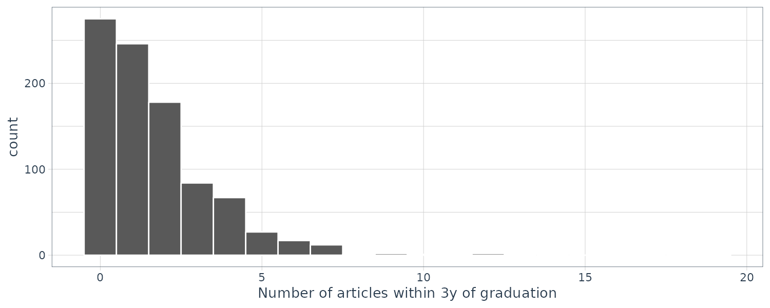
Let’s start with deterimining whether there is a difference in publications between men and women:
> bioChemists |>
group_by(fem) |>
summarize(
counts = sum(art),
n = length(art)
)
# A tibble: 2 × 3
fem counts n
<fct> <int> <int>
1 Men 930 494
2 Women 619 421The hypotheses to compare the two sexes:
\[\begin{aligned} H_{0}: \lambda_{m} &= \lambda_{f}\\ H_{1}: \lambda_{m} &\neq \lambda_{f} \end{aligned}\]\(\lambda\) are the rates of publications.
> poisson.test(
c(930, 619),
T = 3
)
Comparison of Poisson rates
data: c(930, 619) time base: 1
count1 = 930, expected count1 = 774.5, p-value = 0.000000000000002727
alternative hypothesis: true rate ratio is not equal to 1
95 percent confidence interval:
1.355716 1.665905
sample estimates:
rate ratio
1.502423The T argument allows us to account for the time when the events were counted, which was 3 years for both men and women.
The low p-value indicate that the observed difference is greater than noise and favors the alternative hypothesis.
To present the result in a tibble:
> poisson.test(c(930, 619)) |>
tidy()
# A tibble: 1 × 8
estimate statistic p.value parameter conf.low conf.high method alternative
<dbl> <dbl> <dbl> <dbl> <dbl> <dbl> <chr> <chr>
1 1.50 930 2.73e-15 774. 1.36 1.67 Comparison of Poisson rates two.sided Rather than assuming a Poisson distribution, we might not use any distribution assumption and use the bootstrap and permutation tests.
Bootstrap Test
Using the infer package, we can use bootstrap distribution in the following way. First we cacluate the difference in means:
library(infer)
observed <- bioChemists |>
specify(art ~ fem) |>
calculate(
stat = "diff in means",
order = c("Men", "Women")
)
> observed
Response: art (numeric)
Explanatory: fem (factor)
# A tibble: 1 × 1
stat
<dbl>
1 0.412This value can be calculated:
\[\begin{aligned} \frac{930 - 619}{\frac{930 + 619}{2}} &= 0.401 \end{aligned}\]Next, we generate a confidence interval for ths mean by creating a bootstrap distribution via generate():
set.seed(2101)
bootstrapped <- bioChemists |>
specify(art ~ fem) |>
generate(
reps = 2000,
type = "bootstrap"
) |>
calculate(
stat = "diff in means",
order = c("Men", "Women")
)
> bootstrapped
Response: art (numeric)
Explanatory: fem (factor)
# A tibble: 2,000 × 2
replicate stat
<int> <dbl>
1 1 0.467
2 2 0.107
3 3 0.467
4 4 0.308
5 5 0.369
6 6 0.428
7 7 0.272
8 8 0.587
9 9 0.468
10 10 0.432
# ℹ 1,990 more rows
# ℹ Use `print(n = ...)` to see more rows A percentile interval is calculated using:
percentile_ci <- get_ci(bootstrapped)
> percentile_ci
# A tibble: 1 × 2
lower_ci upper_ci
<dbl> <dbl>
1 0.158 0.653We can visualize the confidence interval as well:
visualize(bootstrapped) +
shade_confidence_interval(endpoints = percentile_ci) 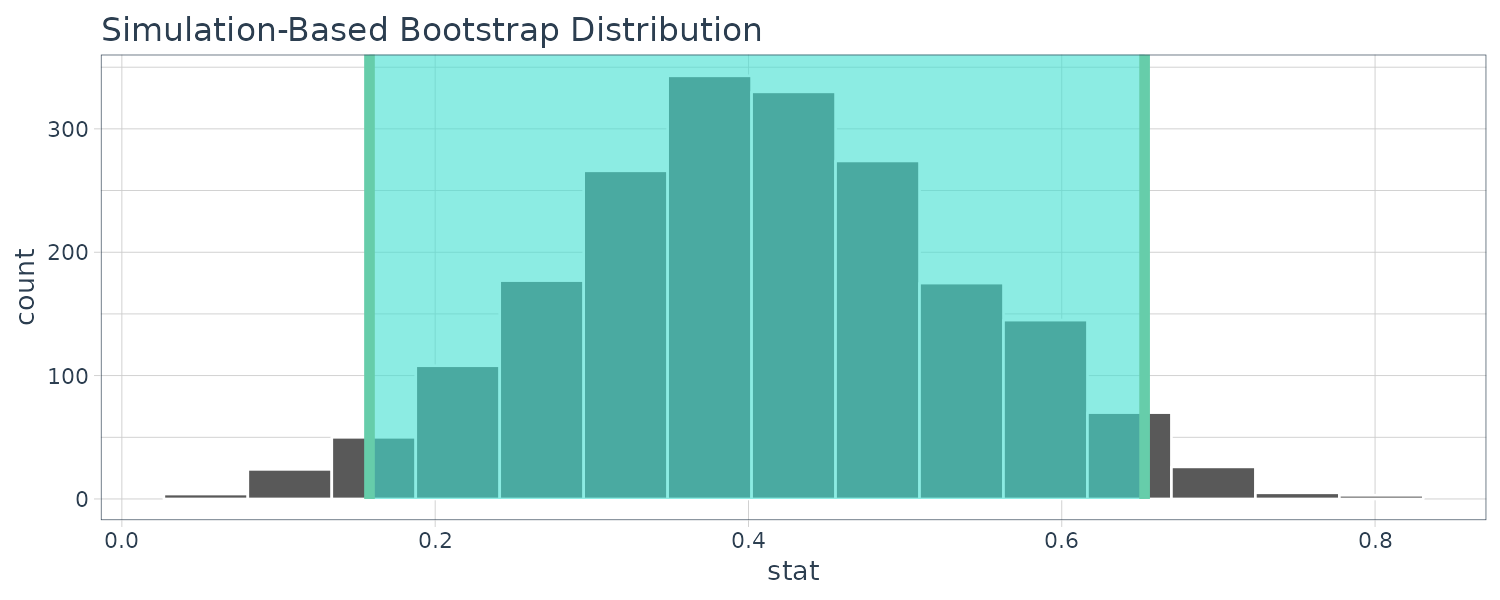
Permutation Test
If we require a p-value, the infer package can compute the value via a permutation test by adding a hypothesize() function call to state the type of assumption to test:
set.seed(2102)
permuted <- bioChemists |>
specify(art ~ fem) |>
hypothesize(null = "independence") |>
generate(
reps = 2000,
type = "permute"
) |>
calculate(
stat = "diff in means",
order = c("Men", "Women")
)
permuted
Response: art (numeric)
Explanatory: fem (factor)
Null Hypothesis: independence
# A tibble: 2,000 × 2
replicate stat
<int> <dbl>
1 1 0.201
2 2 -0.133
3 3 0.109
4 4 -0.195
5 5 -0.00128
6 6 -0.102
7 7 -0.102
8 8 -0.0497
9 9 0.0119
10 10 -0.146
# ℹ 1,990 more rows
# ℹ Use `print(n = ...)` to see more rows
> permuted |>
get_p_value(
obs_stat = observed,
direction = "two-sided"
)
# A tibble: 1 × 1
p_value
<dbl>
1 0.002Similarly, we can visualize the distribution and draw a vertical line to indicate the observed value:
visualize(permuted) +
shade_p_value(obs_stat = observed, direction = "two-sided") 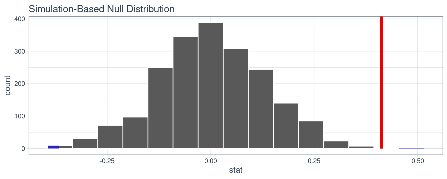
Log-Linear Models
The previous two-sample test are probably suboptimal as they do not account for other factors that might explain the observed relationship between publication rate and set. Let’s move to a more complex model considering additional covariates:
\[\begin{aligned} \log(\lambda) &= \beta_{0} + \beta_{1}x_{1} + \cdots + \beta_{p}x_{p} \end{aligned}\]Where \(\lambda\) is the expected value of the counts. We will fit a Poisson regression model:
library(poissonreg)
log_lin_spec <- poisson_reg()
log_lin_fit <- log_lin_spec |>
fit(
art ~ .,
data = bioChemists
)
> log_lin_fit
parsnip model object
Call: stats::glm(formula = art ~ ., family = stats::poisson, data = data)
Coefficients:
(Intercept) femWomen marMarried kid5 phd ment
0.30462 -0.22459 0.15524 -0.18488 0.01282 0.02554
Degrees of Freedom: 914 Total (i.e. Null); 909 Residual
Null Deviance: 1817
Residual Deviance: 1634 AIC: 3314The tidy() method summarizes the coefficients for the model with 90% CI:
> tidy(
log_lin_fit,
conf.int = TRUE,
conf.level = 0.95
)
# A tibble: 6 × 7
term estimate std.error statistic p.value conf.low conf.high
<chr> <dbl> <dbl> <dbl> <dbl> <dbl> <dbl>
1 (Intercept) 0.305 0.103 2.96 3.10e- 3 0.102 0.505
2 femWomen -0.225 0.0546 -4.11 3.92e- 5 -0.332 -0.118
3 marMarried 0.155 0.0614 2.53 1.14e- 2 0.0352 0.276
4 kid5 -0.185 0.0401 -4.61 4.08e- 6 -0.264 -0.107
5 phd 0.0128 0.0264 0.486 6.27e- 1 -0.0388 0.0647
6 ment 0.0255 0.00201 12.7 3.89e-37 0.0215 0.0294The p-values correspond to separate hypothesis tests for each parameter:
\[\begin{aligned} H_{0}: \beta_{j} &= 0\\ H_{a}: \beta_{j} &\neq 0 \end{aligned}\]To double check the CI, we use the bootstrap confidence intervals for lm() and glm() models:
set.seed(2103)
glm_boot <- rsample::reg_intervals(
art ~ .,
data = bioChemists,
model_fn = "glm",
family = poisson
)
> glm_boot
> # A tibble: 5 × 6
term .lower .estimate .upper .alpha .method
<chr> <dbl> <dbl> <dbl> <dbl> <chr>
1 femWomen -0.358 -0.226 -0.0856 0.05 student-t
2 kid5 -0.298 -0.184 -0.0789 0.05 student-t
3 marMarried 0.000264 0.155 0.317 0.05 student-t
4 ment 0.0182 0.0256 0.0322 0.05 student-t
5 phd -0.0707 0.0130 0.102 0.05 student-t Note that the bootstrap confidence interval is wider than the parametric confidence interval. If the data were truly Poisson, their intervals would have more similar widths.
To determine which predictors to keep, we can conduct the Likelihood Ratio Test (LRT) between nested models. Based on the CI, the predictor phd is statistically insignificant. Let us test the following hypothesis:
\[\begin{aligned} H_{0}: \beta_{phd} &= 0\\ H_{a}: \beta_{phd} &\neq 0 \end{aligned}\]We fit a reduced model and use ANOVA to check for significance:
log_lin_reduced <- log_lin_spec |>
fit(
art ~ ment + kid5 + fem + mar,
data = bioChemists
)
> log_lin_reduced
parsnip model object
Call: stats::glm(formula = art ~ ment + kid5 + fem + mar, family = stats::poisson,
data = data)
Coefficients:
(Intercept) ment kid5 femWomen marMarried
0.34517 0.02576 -0.18499 -0.22530 0.15218
Degrees of Freedom: 914 Total (i.e. Null); 910 Residual
Null Deviance: 1817
Residual Deviance: 1635 AIC: 3312We can tidy the results for the LRT to get the p-value
> anova(
extract_fit_engine(log_lin_reduced),
extract_fit_engine(log_lin_fit),
test = "LRT"
) |>
tidy()
# A tibble: 2 × 6
term df.residual residual.deviance df deviance p.value
<chr> <dbl> <dbl> <dbl> <dbl> <dbl>
1 art ~ ment + kid5 + fem + mar 910 1635. NA NA NA
2 art ~ fem + mar + kid5 + phd + ment 909 1634. 1 0.236 0.627 Zero-Inflated Poisson (ZIP) Model
There are occasions where the number of zero counts is larger than what a simple Poisson distribution would prescribe. The equation for the mean \(\lambda\) is:
\[\begin{aligned} \lambda &= \pi 0 + (1 - \pi)\lambda_{nz}\\ \log(\lambda_{nz}) &= \beta_{0} + \beta_{1}x_{1} + \cdots + \beta_{p}x_{p}\\ \log\Big(\frac{\pi}{1 - \pi}\Big) &= \gamma_{0} + \gamma_{1}z_{1} + \cdots + \gamma_{q}z_{p} \end{aligned}\]The x covariates affect the count values while the z covariates influence the probability of a zero.
Let’s fit a model with a full set of z covariates:
zero_inflated_spec <- poisson_reg() |>
set_engine("zeroinfl")
zero_inflated_fit <- zero_inflated_spec |>
fit(
art ~ fem + mar + kid5 + ment |
fem + mar + kid5 + phd + ment,
data = bioChemists
)
> zero_inflated_fit
parsnip model object
Call:
pscl::zeroinfl(formula = art ~ fem + mar + kid5 + ment | fem + mar + kid5 + phd + ment, data = data)
Count model coefficients (poisson with log link):
(Intercept) femWomen marMarried kid5 ment
0.62116 -0.20907 0.10505 -0.14281 0.01798
Zero-inflation model coefficients (binomial with logit link):
(Intercept) femWomen marMarried kid5 phd ment
-0.60865 0.10931 -0.35292 0.21946 0.01236 -0.13509 We can use another likelihood ratio test to see if the new model terms are helpful:
\[\begin{aligned} H_{0}: \ &\gamma_{1} = 0, \gamma_{2} = 0, \cdots, \gamma_{5} = 0\\ H_{a}: \ &\text{at least one }\gamma \neq 0 \end{aligned}\]But unfortunately, anova() isn’t implemented for zeroinfl objects. Rather, we see which has a higher AIC:
> zero_inflated_fit |>
extract_fit_engine() |>
AIC()
[1] 3231.585
> log_lin_reduced |>
extract_fit_engine() |>
AIC()
[1] 3312.349Note that we are not conducting a formal statistical test but estimating the ability of the data to fit the data. The results indicate that the ZIP model is preferable.
It is better if we can resample a large number of these two models and assess the uncertainty of the AIC statistics. Note that apparent = TRUE creates an additional bootstrap sample with the holdout set the same as training set.
glm_form <- art ~ fem + mar + kid5 + ment
zip_form <- art ~ fem + mar + kid5 + ment |
fem + mar + kid5 + phd + ment
library(purrr)
library(rsample)
set.seed(2104)
bootstrap_models <- bootstraps(
bioChemists,
times = 2000,
apparent = TRUE
) |>
mutate(
glm = map(
splits,
~ fit(
log_lin_spec,
glm_form,
data = analysis(.x)
)
),
zip = map(
splits,
~ fit(
zero_inflated_spec,
zip_form,
data = analysis(.x)
)
)
)
> bootstrap_models
# Bootstrap sampling with apparent sample
# A tibble: 2,001 × 4
splits id glm zip
<list> <chr> <list> <list>
1 <split [915/355]> Bootstrap0001 <fit[+]> <fit[+]>
2 <split [915/333]> Bootstrap0002 <fit[+]> <fit[+]>
3 <split [915/337]> Bootstrap0003 <fit[+]> <fit[+]>
4 <split [915/344]> Bootstrap0004 <fit[+]> <fit[+]>
5 <split [915/351]> Bootstrap0005 <fit[+]> <fit[+]>
6 <split [915/354]> Bootstrap0006 <fit[+]> <fit[+]>
7 <split [915/326]> Bootstrap0007 <fit[+]> <fit[+]>
8 <split [915/336]> Bootstrap0008 <fit[+]> <fit[+]>
9 <split [915/338]> Bootstrap0009 <fit[+]> <fit[+]>
10 <split [915/349]> Bootstrap0010 <fit[+]> <fit[+]>
# ℹ 1,991 more rows
# ℹ Use `print(n = ...)` to see more rows Next we compute the AIC for both models:
bootstrap_models <- bootstrap_models |>
mutate(
glm_aic = map_dbl(
glm,
~ extract_fit_engine(.x) |>
AIC()
),
zip_aic = map_dbl(
zip,
~ extract_fit_engine(.x) |>
AIC()
)
)
> bootstrap_models
# Bootstrap sampling with apparent sample
# A tibble: 2,001 × 6
splits id glm zip glm_aic zip_aic
<list> <chr> <list> <list> <dbl> <dbl>
1 <split [915/355]> Bootstrap0001 <fit[+]> <fit[+]> 3210. 3132.
2 <split [915/333]> Bootstrap0002 <fit[+]> <fit[+]> 3265. 3171.
3 <split [915/337]> Bootstrap0003 <fit[+]> <fit[+]> 3394. 3297.
4 <split [915/344]> Bootstrap0004 <fit[+]> <fit[+]> 3400. 3247.
5 <split [915/351]> Bootstrap0005 <fit[+]> <fit[+]> 3262. 3190.
6 <split [915/354]> Bootstrap0006 <fit[+]> <fit[+]> 3185. 3101.
7 <split [915/326]> Bootstrap0007 <fit[+]> <fit[+]> 3335. 3249.
8 <split [915/336]> Bootstrap0008 <fit[+]> <fit[+]> 3291. 3207.
9 <split [915/338]> Bootstrap0009 <fit[+]> <fit[+]> 3283. 3198.
10 <split [915/349]> Bootstrap0010 <fit[+]> <fit[+]> 3118. 3024.
# ℹ 1,991 more rows
# ℹ Use `print(n = ...)` to see more rows
> mean(bootstrap_models$zip_aic < bootstrap_models$glm_aic)
[1] 1Only one ZIP resample has AIC less than GLM, so it seems definitive that accounting for the excessive number of zero counts is a good idea.
Let’s create a confidence interval for the coefficients and show the first sample:
bootstrap_models <- bootstrap_models |>
mutate(
zero_coefs = map(
zip,
~ tidy(.x, type = "zero")
)
)
> bootstrap_models$zero_coefs[[1]]
# A tibble: 6 × 6
term type estimate std.error statistic p.value
<chr> <chr> <dbl> <dbl> <dbl> <dbl>
1 (Intercept) zero -0.128 0.497 -0.257 0.797
2 femWomen zero -0.0764 0.319 -0.240 0.811
3 marMarried zero -0.112 0.365 -0.307 0.759
4 kid5 zero 0.270 0.186 1.45 0.147
5 phd zero -0.178 0.132 -1.35 0.177
6 ment zero -0.123 0.0315 -3.91 0.0000935 Let’s visualize the bootstrap distribution of the coefficients:
bootstrap_models |>
unnest(zero_coefs) |>
ggplot(aes(x = estimate)) +
geom_histogram(
bins = 25,
color = "white"
) +
facet_wrap(
~term,
scales = "free_x"
) +
geom_vline(
xintercept = 0,
lty = 2,
color = "gray70"
) +
theme_tq()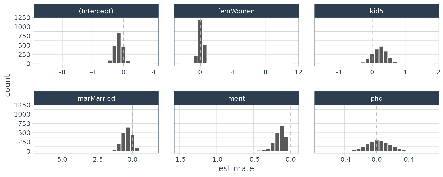
We can compute the bootstrap confidence interval and t-distribution confidence interval. The rsample package contains a set of functions named int_*() that compute different types of bootstrap intervals (standard percentil and t-distribution):
> bootstrap_models |>
int_pctl(zero_coefs)
# A tibble: 6 × 6
term .lower .estimate .upper .alpha .method
<chr> <dbl> <dbl> <dbl> <dbl> <chr>
1 (Intercept) -1.75 -0.621 0.423 0.05 percentile
2 femWomen -0.521 0.115 0.818 0.05 percentile
3 kid5 -0.327 0.218 0.677 0.05 percentile
4 marMarried -1.20 -0.381 0.362 0.05 percentile
5 ment -0.401 -0.162 -0.0513 0.05 percentile
6 phd -0.276 0.0220 0.327 0.05 percentile
> bootstrap_models |>
int_t(zero_coefs)
# A tibble: 6 × 6
term .lower .estimate .upper .alpha .method
<chr> <dbl> <dbl> <dbl> <dbl> <chr>
1 (Intercept) -1.61 -0.621 0.321 0.05 student-t
2 femWomen -0.482 0.115 0.671 0.05 student-t
3 kid5 -0.211 0.218 0.599 0.05 student-t
4 marMarried -0.988 -0.381 0.290 0.05 student-t
5 ment -0.324 -0.162 -0.0275 0.05 student-t
6 phd -0.274 0.0220 0.291 0.05 student-tFrom this, we can get a pretty good idea which predictors to include in the ZIP model.
See Also
References
Kuhn M., Silge J. (2022), Tidy Modeling with R: A Framework for Modeling in the Tidyverse
