Time Series Analysis - Spectral Analysis
Read PostIn this post, we will continue with Shumway H. (2017) Time Series Analysis, focusing on Spectral Analysis. We will look into the frequency domain approach to time series analysis. We argue that the concept of regularity of a series can best be expressed in terms of periodic variations of the underlying phenomenon that produced the series.
Contents:
Cyclical Behavior and Periodicity
In order to define the rate at which a series oscillates, we first define a cycle as one complete period of a sine or cosine function defined over a unit time interval.
Consider the periodic process:
\[\begin{aligned} x_{t} &= A \mathrm{cos}(2\pi \omega t + \phi) \end{aligned}\]Where \(\omega\) is a frequency index, defined in cycles per unit time. Using trigonometric identity, we can rewrite \(x_{t}\) as:
\[\begin{aligned} x_{t} &= U_{1}\textrm{cos}(2\pi \omega t) + U_{2}\textrm{sin}(2\pi \omega t) \end{aligned}\] \[\begin{aligned} U_{1} &= A\ \mathrm{cos}(\phi)\\ U_{2} &= -A\ \mathrm{sin}(\phi) \end{aligned}\]\(U_{1}, U_{2}\) are often taken to be normally distributed random variables. In this case:
\[\begin{aligned} A &= \sqrt{U_{1}^{2} + U_{2}^{2}}\\ \phi &= \mathrm{tan}^{-1}\Big(\frac{-U_{2}}{U_{1}}\Big) \end{aligned}\]\(A, \phi\) are independent random variables iff:
\[\begin{aligned} A^{2} &\sim \chi^{2}(2) \end{aligned}\] \[\begin{aligned} \phi &\sim U(-\pi, \pi) \end{aligned}\]Assuming \(U_{1}, U_{2}\) are uncorrelated random variables with mean 0 and variance \(\sigma^{2}\) then:
\[\begin{aligned} c_{t} &= \mathrm{cos}(2\pi\omega t)\\ s_{t} &= \mathrm{sin}(2\pi\omega t) \end{aligned}\] \[\begin{aligned} \gamma_{x}(h) &= \text{cov}(x_{t+h}, x_{t})\\ &= \text{cov}(U_{1}c_{t+h} + U_{2}s_{t+h}, U_{1}c_{t} + U_{2}s_{t})\\ &= E[(U_{1}c_{t+h} + U_{2}s_{t+h})(U_{1}c_{t} + U_{2}s_{t})]\\ &= E[U_{1}c_{t+h}U_{1}c_{t} + U_{1}c_{t+h}U_{2}s_{t} + U_{2}s_{t+h}U_{1}c_{t} + U_{2}s_{t+h}U_{2}s_{t}]\\ &= \sigma^{2}c_{t+h}c_{t} + 0 + 0 + \sigma^{2}s_{t+h}s_{t}\\ &= \sigma^{2}c_{t+h}c_{t} + \sigma^{2}s_{t+h}s_{t}\\ \end{aligned}\]Using the identity:
\[\begin{aligned} \text{cos}(\alpha \pm \beta) &= \mathrm{cos}(\alpha)\mathrm{cos}(\beta) \mp \mathrm{sin}(\alpha)\mathrm{sin}(\beta) \end{aligned}\] \[\begin{aligned} \gamma_{x}(h) &= \sigma^{2}c_{t+h}c_{t} + \sigma^{2}s_{t+h}s_{t}\\ &= \sigma^{2}\textrm{cos}(2\pi\omega h) \end{aligned}\]And:
\[\begin{aligned} \text{var}(x_{t}) &= \gamma_{x}(0)\\ &= \sigma^{2}\textrm{cos}(2\pi\omega \times 0)\\ &= \sigma^{2} \end{aligned}\]To find the sample variance, we take the sample variance of the two observations:
\[\begin{aligned} S^{2} &= \frac{\hat{U}_{1}^{2} + \hat{U}_{2}^{2}}{2 - 1}\\[5pt] &= \hat{U}_{1}^{2} + \hat{U}_{2}^{2} \end{aligned}\]In general, for data that occur at discrete time points, we need at least 2 points to determine a cycle, so the highest frequency is 0.5 cycles per point. For example, if \(\omega = 0.5\), a cycle take two unit time. And that is the highest frequency we can detect if sample at each unit time point. This frequency is known as the folding frequency and defines the highest frequency that can be seen in discrete sampling.
Higher frequencies sampled this way will appear at lower frequencies, called aliases.
Now consider a mixture of periodic series with multiple frequencies and amplitudes:
\[\begin{aligned} x_{t} &= \sum_{k = 1}^{q}U_{k1}\mathrm{cos}(2\pi\omega_{k}t) + U_{k2}\mathrm{sin}(2\pi\omega_{k}t) \end{aligned}\]Where \(U_{k1}, U_{k2}\) are uncorrelated zero-mean random variables with variance \(\sigma_{k}^{2}\) and \(\omega_{k}\) are distinct frequencies.
We can show that the autocovariance function is:
\[\begin{aligned} \gamma_{x}(h) &= \sum_{k=1}^{q}\sigma_{k}^{2}\mathrm{cos}(2\pi\omega_{k}h)\\ \gamma_{x}(0) &= \text{var}(x_{t})\\ &= \sum_{k=1}^{q}\sigma_{k}^{2} \end{aligned}\]And the sum of the sample variances:
\[\begin{aligned} \hat{\gamma}_{x}(0) &= \sum_{k=1}^{q}\frac{\hat{U}_{k1}^{2} + \hat{U}_{k2}^{2}}{2 - 1} \end{aligned}\]Example: A Periodic Series
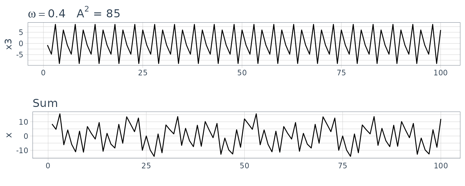
We will generate the following series in R:
\[\begin{aligned} x_{t1} &= 2 \mathrm{cos}\Big(2\pi t\times\frac{6}{100} \Big) + 3 \mathrm{sin}\Big(2\pi t\times\frac{6}{100} \Big)\\[5pt] x_{t2} &= 4 \mathrm{cos}\Big(2\pi t\times\frac{10}{100} \Big) + 5 \mathrm{sin}\Big(2\pi t\times\frac{10}{100} \Big)\\[5pt] x_{t3} &= 6 \mathrm{cos}\Big(2\pi t\times\frac{40}{100} \Big) + 7 \mathrm{sin}\Big(2\pi t\times\frac{40}{100} \Big) \end{aligned}\]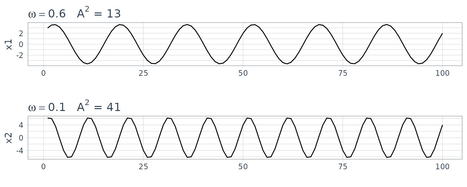
Example: Estimation and the Periodogram
Consider a time series sample, \(x_{1}, \cdots, x_{n}\) where n is odd:
\[\begin{aligned} x_{t} &= a_{0} + \sum_{j=1}^{\frac{n-1}{2}}a_{j}\textrm{cos}\Big(\frac{2\pi tj}{n}\Big) + b_{j}\textrm{sin}\Big(\frac{2\pi tj}{n}\Big) \end{aligned}\] \[\begin{aligned} t &= 1, \cdots, n \end{aligned}\]Or when n is even:
\[\begin{aligned} x_{t} &= a_{0} + a_{\frac{n}{2}}\textrm{cos}\Big(\frac{2\pi t}{2}\Big) + \sum_{j=1}^{\frac{n}{2} - 1}a_{j}\textrm{cos}\Big(\frac{2\pi tj}{n}\Big) + b_{j}\textrm{sin}\Big(\frac{2\pi tj}{n}\Big)\\ \end{aligned}\]Using OLE estimation, the coefficients are:
\[\begin{aligned} a_{0} &= \bar{x}\\ a_{j} &= \frac{2}{n}\sum_{t=1}^{n}x_{t}\mathrm{cos}\Big(\frac{2\pi t j}{n}\Big)\\[5pt] b_{j} &= \frac{2}{n}\sum_{t=1}^{n}x_{t}\mathrm{sin}\Big(\frac{2\pi t j}{n}\Big) \end{aligned}\]We then define the scaled periodgram as:
\[\begin{aligned} P\Big(\frac{j}{n}\Big) &= a_{j}^{2} + b_{j}^{2} \end{aligned}\]This is simply the sample variance at each frequency component and is an estimate of \(\sigma_{j}^{2}\) corresponding to the frequency of \(\omega_{j} = \frac{j}{n}\). These frequencies are known as Fourier/fundamental frequencies.
It is not necessary to run a large regression to obtain \(a_{j}, b_{j}\) and they can be computed quickly if n is a highly composite integer (if not can pad with zeros).
The Discrete Fourier Transform (DFT) is a complex-valued weighted average of the data given by:
\[\begin{aligned} d\Big(\frac{j}{n}\Big) &= \frac{1}{\sqrt{n}}\sum_{t=1}^{n}x_{t}e^{-\frac{2\pi i t j}{n}}\\ &= \frac{1}{\sqrt{n}}\sum_{t=1}^{n}x_{t}\textrm{cos}\Big(\frac{2\pi t j}{n}\Big) - i\sum_{t=1}^{n}x_{t}\textrm{sin}\Big(\frac{2\pi t j}{n}\Big) \end{aligned}\] \[\begin{aligned} j &= 0, 1, \cdots, n - 1 \end{aligned}\]Where \(\frac{j}{n}\) are the Fourier frequencies.
Because of a large number of redundancies in the calculation, the above can be computed quicker using the FFT.
For example, in R:
dft <- fft(x) / sqrt(length(x))
idft <- fft(dft, inverse = TRUE) / sqrt(length(dft))
Note that the periodogram is:
\[\begin{aligned} \Big|d\Big(\frac{j}{n}\Big)\Big|^{2} &= \frac{1}{n}\Bigg(\sum_{t=1}^{n}x_{t}\mathrm{cos}\Big(\frac{2\pi t j}{n}\Big)\Bigg)^{2} + \frac{1}{n}\Bigg(\sum_{t=1}^{n}x_{t}\mathrm{sin}\Big(\frac{2\pi t j}{n}\Big)\Bigg)^{2} \end{aligned}\]And the scaled periodogram can be calculated as:
\[\begin{aligned} P\Big(\frac{j}{n}\Big) &= \frac{4}{n}\Big|d\Big(\frac{j}{n}\Big)\Big|^{2} \end{aligned}\]And note that there is a mirroring effect at the folding frequency of \(\frac{1}{2}\):
\[\begin{aligned} P\Big(\frac{j}{n}\Big) &= P\Big(1 - \frac{j}{n}\Big) \end{aligned}\] \[\begin{aligned} j &= 0, 1, \cdots, n-1 \end{aligned}\]Calculating the scaled periodogram in R (note that R does not include the factor \(\frac{1}{\sqrt{n}}\) in fft()):
n <- 100
dat$P <- 4 / n *
  Mod(fft(dat$x) / sqrt(n))^2
dat$freq <- 0:99 / 100

> dat |>
  ggplot(aes(x = freq, y = P)) +
  geom_segment(
    aes(
      x = freq,
      xend = freq,
      y = 0,
      yend = P
    )
  ) +
  theme_tq()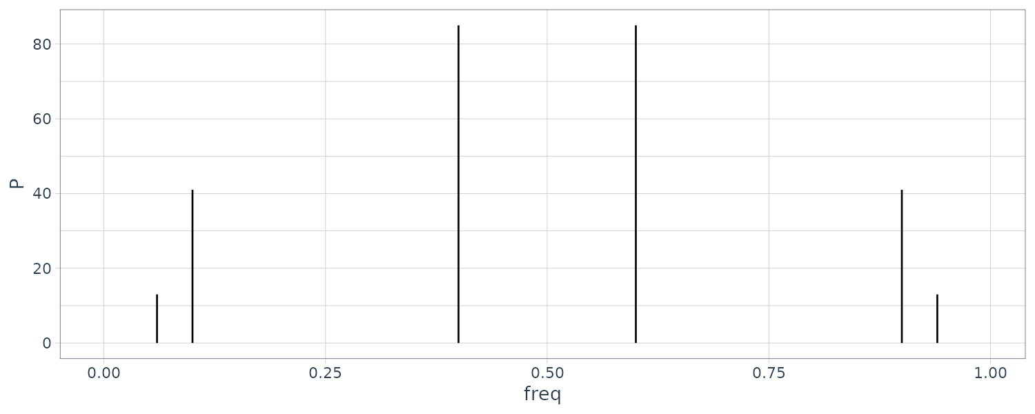
From R we can see the 3 frequencies in the periodogram:
\[\begin{aligned} P\Big(\frac{6}{100}\Big) &= P\Big(\frac{6}{100}\Big) = 13\\ P\Big(\frac{10}{100}\Big) &= P\Big(\frac{10}{100}\Big) = 41\\ P\Big(\frac{40}{100}\Big) &= P\Big(\frac{40}{100}\Big) = 85 \end{aligned}\]Otherwise:
\[\begin{aligned} P\Big(\frac{j}{100}\Big) &= 0 \end{aligned}\]> dat$P[6 + 1]
[1] 13
> dat$P[(100 - 6) + 1]
[1] 13
> dat$P[10 + 1]
[1] 41
> dat$P[(100 - 10) + 1]
[1] 41
> dat$P[40 + 1]
[1] 85
> dat$P[(100 - 40) + 1]
[1] 85Example: Star Magnitude
The star dataset which contain the magnitude of a star taken at midnight for 600 consecutive days. The two most prominent periodic components in the periodogram are the 29 and 24 day cycle:
star <- as_tsibble(star)

n <- nrow(star)
dat <- tibble(
  P = P <- 4 / n *
    Mod(fft(star$value - mean(star$value)) / sqrt(n))^2,
  freq = (0:(n - 1)) / n
)

dat |>
  slice(1:50) |>
  ggplot(aes(x = freq, y = P)) +
  geom_segment(
    aes(
      x = freq,
      xend = freq,
      y = 0,
      yend = P
    )
  ) +
  annotate("text", label = "24 day cycle", x = 0.047, y = 62) +
  annotate("text", label = "29 day cycle", x = 0.03, y = 74) +
  theme_tq()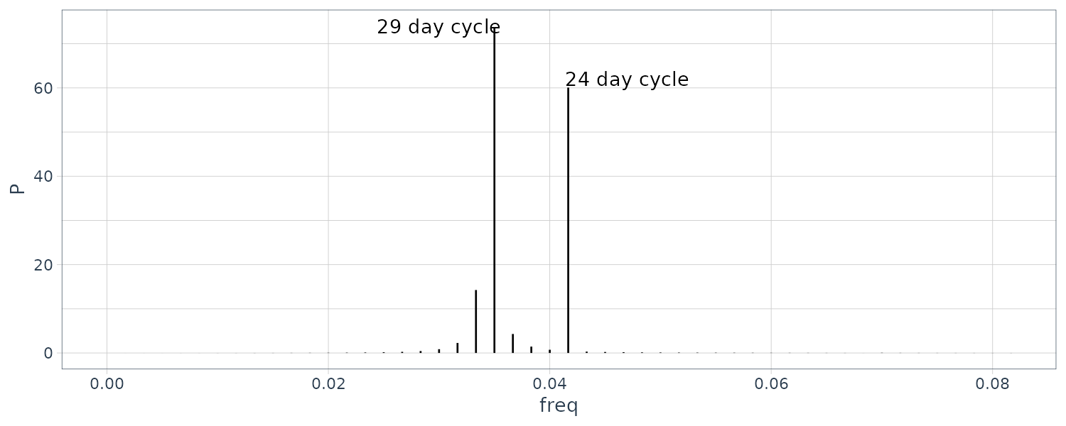
freqs <- dat |>
  slice(1:50) |>
  arrange(desc(P)) |>
  slice(1:2) |>
  pull(freq)

> freqs
[1] 0.03500000 0.04166667

> 1 / freqs
[1] 28.57143 24.00000
Spectral Density
In this section, we define the fundamental frequency domain tool, the spectral density. In addition, we discuss the spectral representations for stationary processes. Just as the Wold decomposition theoretically justified the use of regression for analyzing time series, the spectral representation theorems supply the theoretical justifications for decomposing stationary time series into periodic components appearing in proportion to their underlying variances.
Consider the following periodic stationary random process:
\[\begin{aligned} x_{t} = U_{1}\mathrm{cos}(2\pi \omega_{0}t) + U_{2}\mathrm{sin}(2\pi \omega_{0}t) \end{aligned}\]Recall that:
\[\begin{aligned} \gamma(h) &= \sigma^{2}\mathrm{cos}(2\pi\omega_{0}h) \end{aligned}\]Using Euler’s formula for cosine:
\[\begin{aligned} \mathrm{cos}(\alpha) &= \frac{e^{i\alpha} + e^{-i\alpha}}{2} \end{aligned}\] \[\begin{aligned} \gamma(h) &= \sigma^{2}\mathrm{cos}(2\pi\omega_{0}h)\\ &= \frac{\sigma^{2}}{2}e^{-2\pi i \omega_{0}h} + \frac{\sigma^{2}}{2}e^{2\pi i \omega_{0}h} \end{aligned}\]And using Riemann-Stieltjes integration, we can show:
\[\begin{aligned} \gamma(h) &= \sigma^{2}\mathrm{cos}(2\pi\omega_{0}h)\\[5pt] &= \frac{\sigma^{2}}{2}e^{-2\pi i \omega_{0}h} + \frac{\sigma^{2}}{2}e^{2\pi i \omega_{0}h}\\[5pt] &= \int_{-\frac{1}{2}}^{\frac{1}{2}}e^{2\pi i \omega h}\ dF(\omega) \end{aligned}\]Where \(F(\omega)\) is defined as:
\[\begin{aligned} F(\omega) &= \begin{cases} 0 & \omega < -\omega_{0}\\ \frac{\sigma^{2}}{2} & -\omega_{0} < \omega < \omega_{0}\\ \sigma^{2} & \omega \geq \omega_{0}\\ 0 & h > 1 \end{cases} \end{aligned}\]\(F(\omega)\) is a cumulative distribution function of variances. Hence, we term \(F(\omega)\) as the spectral distribution function.
Spectral Representation of an Autocovariance Function
If \(\{x_{t}\}\) is stationary with \(\gamma(h) = \text{cov}(x_{t+h}, x_{t})\), then there exists a unique monotonically increasing spectral distribution function \(F(\omega)\):
\[\begin{aligned} F(-\infty) &= F\Big(-\frac{1}{2}\Big) = 0\\ F(\infty) &= F\Big(\frac{1}{2}\Big) = \gamma(0)\\ \gamma(h) &= \int_{-\frac{1}{2}}^{\frac{1}{2}}e^{2\pi i \omega h}\ dF(\omega) \end{aligned}\]If the autocovariance function further satisfies:
\[\begin{aligned} \sum_{h =-\infty}^{\infty}| \gamma(h)| < \infty \end{aligned}\]Then it has the spectral representation:
\[\begin{aligned} \gamma(h) &= \int_{-\frac{1}{2}}^{\frac{1}{2}}e^{2\pi i \omega h}f(\omega)\ d\omega\\[5pt] h &= 0, \pm 1, \pm 2, \cdots \end{aligned}\]And the inverse transform of the spectral density:
\[\begin{aligned} f(\omega) &= \sum_{h=-\infty}^{\infty}\gamma(h)e^{-2\pi i \omega h}\\ \end{aligned}\] \[\begin{aligned} - \frac{1}{2} \leq \omega \leq \frac{1}{2} \end{aligned}\]The spectral density is the analogue of the pdf and:
\[\begin{aligned} f(\omega) &\geq 0 \end{aligned}\] \[\begin{aligned} f(\omega) &= f(-\omega) \end{aligned}\]The variance is the integrated spectral density over all of the frequencies:
\[\begin{aligned} \gamma(0) &= \text{var}(x_{t})\\ &= \int_{-\frac{1}{2}}^{\frac{1}{2}}f(\omega)\ d\omega \end{aligned}\]The autocovariance and the spectral distribution functions contain the same information. That information, however, is expressed in different ways. The autocovariance function expresses information in terms of lags, whereas the spectral distribution expresses the same information in terms of cycles.
Some problems are easier to work with when considering lagged information and we would tend to handle those problems in the time domain. Nevertheless, other problems are easier to work with when considering periodic information and we would tend to handle those problems in the spectral domain.
We note that the autocovariance function, \(\gamma(h)\), and the spectral density, \(f(\omega)\), are Fourier transform pairs. In particular, this means that if \(f(\omega)\) and \(g(\omega)\) are two spectral densities for which:
\[\begin{aligned} \gamma_{f}(h) &= \int_{-\frac{1}{2}}^{\frac{1}{2}}f(\omega)e^{2\pi i \omega h}\ d\omega\\ &= \int_{-\frac{1}{2}}^{\frac{1}{2}}g(\omega)e^{2\pi i \omega h}\ d\omega\\ &= \gamma_{g}(h) \end{aligned}\]Then:
\[\begin{aligned} f(\omega) &= g(\omega) \end{aligned}\]Example: White Noise Series
Recall the variance of white noise is:
\[\begin{aligned} \gamma(0) &= \int_{-\frac{1}{2}}^{\frac{1}{2}}f(\omega)d\omega\\ &= \sigma_{\omega}^{2} \end{aligned}\]And:
\[\begin{aligned} f(\omega) &= \sum_{h=-\infty}^{\infty}\gamma(h)e^{-2\pi i \omega h}\\ &= \gamma(0) + 0 + \cdots\\ &= \sigma_{\omega}^{2} \end{aligned}\]Hence the process contains equal power at all frequencies. The name white noise comes from the analogy to white light.
Output Spectrum of a Filtered Stationary Series
A linear filter uses a set of specified coefficients \(a_{j}\) to transform an input series \(x_{t}\) to \(y_{t}\):
\[\begin{aligned} y_{t} &= \sum_{j=-\infty}^{\infty}a_{j}x_{t-j} \end{aligned}\] \[\begin{aligned} \sum_{j=-\infty}^{\infty}| a_{j}| &< \infty \end{aligned}\]This form is also called a convolution and coefficients are called the impulse response function.
The Fourier transform is called the frequency response function:
\[\begin{aligned} A(\omega) &= \sum_{j=-\infty}^{\infty}a_{j}e^{-2\pi i \omega j} \end{aligned}\]If \(x_{t}\) has a spectrum \(f_{x}(\omega)\), then the spectrum of the ouput \(y_{t}\) is:
\[\begin{aligned} f_{y}(\omega) &= | A(\omega)| ^{2}f_{x}(\omega) \end{aligned}\]The Spectral Density of ARMA
If \(x_{t}\) is ARMA, then:
\[\begin{aligned} x_{t} &= \sum_{j=0}^{\infty}\psi_{j}w_{t-j} \end{aligned}\] \[\begin{aligned} \sum_{j=0}^{\infty}| \psi_{j}| < \infty \end{aligned}\]We know that the spectral density for white noise:
\[\begin{aligned} f_{\omega}(\omega) &= \sigma_{\omega}^{2}\\ \psi(z) &= \frac{\theta(z)}{\phi(z)} \end{aligned}\]We can show that the spectral density for ARMA(p, q) \(x_{t}\):
\[\begin{aligned} f_{x}(\omega) &= \sigma_{\omega}^{2}\frac{|\theta(e^{-2\pi i \omega})|^{2}}{|\phi(e^{-2\pi i \omega})|^{2}} \end{aligned}\] \[\begin{aligned} \phi(z) &= 1 - \sum_{k=1}^{p}\phi_{k}z^{k}\\ \theta(z) &= 1 + \sum_{k=1}^{1}\theta_{k}z^{k}\\ A(\omega) &= \frac{\theta(e^{-2\pi i \omega})}{\phi(e^{-2\pi i \omega})} \end{aligned}\]Example: Moving Average
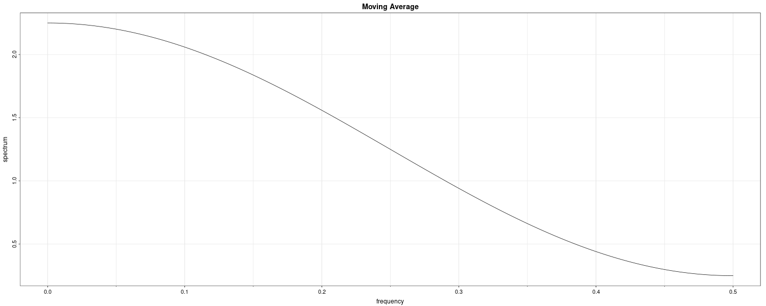
Consider the MA(1) model:
\[\begin{aligned} x_{t} = w_{t} + 0.5w_{t-1} \end{aligned}\]The autocovariance function:
\[\begin{aligned} \gamma(0) &= (1 + 0.5^{2})\sigma_{w}^{2}\\ &= 1.25\sigma_{w}^{2}\\ \end{aligned}\] \[\begin{aligned} \gamma(\pm 1) &= 0.5\sigma_{w}^{2}\\[5pt] \gamma(\pm h) &= 0\\[5pt] h &> 1 \end{aligned}\]The spectral density:
\[\begin{aligned} f_{x}(\omega) &= \sum_{h=-\infty}^{\infty}\gamma(h)e^{-2\pi i \omega h}\\ &= \sigma_{w}^{2}[1.25 + 0.5(e^{-2\pi i \omega} + e^{2\pi i \omega})]\\ &= \sigma_{w}^{2}[1.25 + \textrm{cos}(2\pi \omega)] \end{aligned}\]Computing the spectral density in a different way:
\[\begin{aligned} f_{x}(\omega) &= \sigma_{\omega}^{2}\frac{|\theta(e^{-2\pi i \omega})|^{2}}{|\phi(e^{-2\pi i \omega})|^{2}}\\[5pt] &= \sigma_{w}^{2}|1 + 0.5e^{-2\pi i \omega}|^{2}\\ &= \sigma_{w}^{2}(1 + 0.5e^{-2\pi i \omega})(1 + 0.5e^{-2\pi i \omega})\\ &= \sigma_{w}^{2}[1.25 + 0.5(e^{-2\pi i \omega} + e^{2\pi i \omega})]\\ &= \sigma_{w}^{2}[1.25 + \textrm{cos}(2\pi \omega)] \end{aligned}\] \[\begin{aligned} \theta(z) &= 1 + 0.5z \end{aligned}\]We can plot the spectral density in R:
library(astsa)
arma.spec(
  ma = .5,
  main = "Moving Average"
)
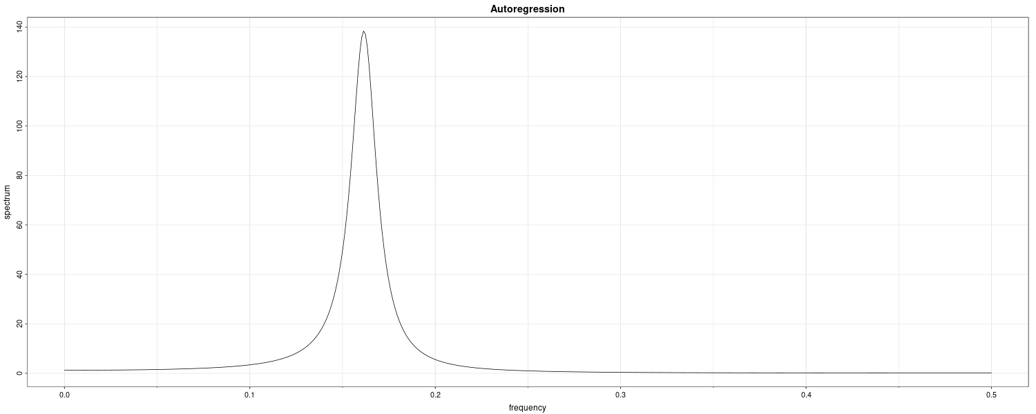
Example: An AR(2) Model
Consider an AR(2) model:
\[\begin{aligned} x_{t} - x_{t-1} + 0.9x_{t-2} = w_{t} \end{aligned}\]Note that:
\[\begin{aligned} \theta(z) &= 1\\ \phi(z) &= 1 - z + 0.9z^{2} \end{aligned}\]Hence:
\[\begin{aligned} |\phi(e^{-2\pi i \omega})|^{2} &= (1 - e^{-2\pi i \omega} + 0.9e^{-4\pi i \omega})(1 - e^{-2\pi i \omega} + 0.9e^{-4\pi i \omega})\\ &= 2.81 - 1.9(e^{2\pi i \omega} + e^{-2\pi i \omega}) + 0.9(e^{4\pi i \omega} + e^{-4\pi i \omega})\\ &= 2.81 - 3.8\mathrm{cos}(2\pi\omega) + 1.8\mathrm{cos}(4\pi\omega) \end{aligned}\] \[\begin{aligned} f_{x}(\omega) &= \frac{\sigma_{w}^{2}}{2.81 - 3.8\mathrm{cos}(2\pi\omega) + 1.8\mathrm{cos}(4\pi\omega)} \end{aligned}\]Graphing this in R:
arma.spec(
  ar = c(1, -0.9),
  main = "Autoregression"
)
Example: Every Explosion has a Cause
Suppose that:
\[\begin{aligned} x_{t} &= 2 x_{t-1} + w_{t}\\ w_{t} &\sim N\Big(0, \sigma_{w}^{2}\Big) \end{aligned}\]The spectral density of x_{t} is:
\[\begin{aligned} w_{t} &= x_{t} - 2x_{t-1}\\ A(\omega) &= 1 - 2e^{-2\pi i \omega}\\ f_{w}(\omega) &= |A(\omega)|^{2}f_{x}(\omega)\\ f_{x}(\omega) &= \frac{1}{|A(\omega)|^{2}}f_{w}(\omega)\\ &= \sigma_{w}^{2}|1 - 2e^{-2\pi i \omega}|^{-2} \end{aligned}\]But:
\[\begin{aligned} |1 - 2^{-2\pi i \omega}| &= |1 - 2^{2\pi i \omega}|\\ &= \Big|(2e^{2\pi i \omega})\Big(\frac{1}{2}e^{-2\pi i \omega} - 1\Big)\Big| \end{aligned}\]Thus, we can rewrite:
\[\begin{aligned} f_{x}(\omega) &= \frac{1}{4}\sigma_{w}^{2}\Big|1 - \frac{1}{2}e^{-2\pi i \omega}\Big|^{-2}\\ x_{t} &= \frac{1}{2}x_{t-1} + v_{t}\\ v_{t} &\sim N\Big(0, \frac{1}{4}\sigma_{w}^{2}\Big) \end{aligned}\]Discrete Fourier Transform
Given data \(x_{1}, \cdots, x_{n}\), we define the DFT to be:
\[\begin{aligned} d(\omega_{j}) &= \frac{1}{\sqrt{n}}\sum_{t=1}^{n}x_{t}e^{-2\pi i \omega_{j}t} \end{aligned}\] \[\begin{aligned} j &= 0, 1, \cdots, n-1 \end{aligned}\] \[\begin{aligned} \omega_{j} &= \frac{j}{n} \end{aligned}\]\(\omega_{j}\) are called the Fourier or fundamental frequencies.
If n is a highly composite integer (it has many factors), the DFT can be computed by FFT.
The inverse DFT:
\[\begin{aligned} x_{t} &= \frac{1}{\sqrt{n}}\sum_{j=0}^{n-1}d(\omega_{j})e^{2\pi i \omega_{j}t} \end{aligned}\]We define the periodogram to be:
\[\begin{aligned} I(\omega_{j}) &= |d(\omega_{j})|^{2} \end{aligned}\] \[\begin{aligned} j &= 0, 1, \cdots, n-1 \end{aligned}\]Note that:
\[\begin{aligned} I(0) &= n\bar{x}^{2} \end{aligned}\]The periodgram can be viewed as the sample spectral density of \(x_{t}\):
\[\begin{aligned} I(\omega_{j}) &= |d(\omega_{j})|^{2}\\ &= \frac{1}{\sqrt{n}}\sum_{t=1}^{n}x_{t}e^{-2\pi i \omega_{j}t}\frac{1}{\sqrt{n}}\sum_{s=1}^{n}x_{s}e^{-2\pi i \omega_{j}s}\\ &= \frac{1}{n}\sum_{t=1}^{n}\sum_{s=1}^{n}x_{t}x_{s}e^{-2\pi i \omega (t-s)}\\ &= \frac{1}{n}\sum_{h=-(n-1)}^{n-1}\sum_{t=1}^{n-|h|}x_{t+|h|}x_{t}e^{-2\pi i \omega_{j} h}\\ &= \sum_{h=-(n-1)}^{n-1}\hat{\gamma(h)}e^{-2\pi i \omega_{j} h} \end{aligned}\]It is sometimes useful to work with the real and imaginary parts of the DFT individually.
We defined the cosine transform as:
\[\begin{aligned} d_{c}(\omega_{j}) &= \frac{1}{\sqrt{n}}\sum_{t=1}^{n}\textrm{cos}(2\pi\omega_{j}t) \end{aligned}\]And the sine transform:
\[\begin{aligned} d_{s}(\omega_{j}) &= \frac{1}{\sqrt{n}}\sum_{t=1}^{n}\textrm{sin}(2\pi\omega_{j}t) \end{aligned}\] \[\begin{aligned} \omega_{j} &= \frac{j}{n} \end{aligned}\] \[\begin{aligned} j &= 0, 1, \cdots, n-1 \end{aligned}\]Note that:
\[\begin{aligned} d(\omega_{j}) &= d_{c}(w_{j})- i d_{s}(\omega_{j})\\[5pt] I(\omega_{j}) &= d_{c}^{2}(\omega_{j}) + d_{s}^{2}(\omega_{j}) \end{aligned}\]Example: Spectral ANOVA
We have also discussed the fact that spectral analysis can be thought of as an analysis of variance.
Recall that we assumed previously that:
\[\begin{aligned} x_{t} &= a_{0} + \sum_{j=1}^{\frac{n-1}{2}}a_{j}\textrm{cos}(2\pi \omega_{j}t) + b_{j}\textrm{sin}(2\pi \omega_{j}t)\\ \end{aligned}\] \[\begin{aligned} t &= 1, \cdots, n \end{aligned}\]Using multiple regression, we could show that the coefficients are:
\[\begin{aligned} a_{0} &= \bar{x} \end{aligned}\] \[\begin{aligned} a_{j} &= \frac{2}{n}\sum_{t=1}^{n}x_{t}\textrm{cos}(2\pi \omega_{j}t)\\ &= \frac{2}{\sqrt{n}}d_{c}(\omega_{j})\\ b_{j} &= \frac{2}{n}\sum_{t=1}^{n}x_{t}\textrm{sin}(2\pi \omega_{j}t)\\ &= \frac{2}{\sqrt{n}}d_{s}(\omega_{j}) \end{aligned}\]Hence:
\[\begin{aligned} (x_{t} - \bar{x}) &= \frac{2}{\sqrt{n}}\sum_{j=1}^{\frac{n-1}{2}}[d_{c}(\omega_{j})\textrm{cos}(2\pi \omega_{j}t) + d_{s}(\omega_{j})\textrm{sin}(2\pi \omega_{j}t)] \end{aligned}\] \[\begin{aligned} t & = 1, \cdots, n \end{aligned}\]Squaring both sides and summing:
\[\begin{aligned} \sum_{t=1}^{n}(x_{t} - \bar{x})^{2} &= 2\sum_{j=1}^{\frac{n-1}{2}}[d_{c}^{2}(\omega_{j}) + d_{s}^{2}(\omega_{j})]\\ &= 2 \sum_{j=1}^{\frac{n-1}{2}}I(\omega_{j}) \end{aligned}\]Thus, we have partitioned the sum of squares into harmonic components represented by frequency \(\omega_{j}\) with the periodogram, \(I(\omega_{j})\), being the mean square regression.
We expect the SSS for the coefficients \(\omega_{1}, \cdots, \omega_{\frac{n-1}{2}}\) to be:
\[\begin{aligned} 2I&(\omega_{1})\\ 2I&(\omega_{2})\\ &\vdots\\ 2I(&\omega_{\frac{n-1}{2}}) \end{aligned}\]And MSE:
\[\begin{aligned} I&(\omega_{1})\\ I&(\omega_{2})\\ &\vdots\\ I(&\omega_{\frac{n-1}{2}}) \end{aligned}\]Example: Spectral Analysis as Principal Component Analysis
If \(X = (x_{1}, \cdots, x_{n})\) are n values of a mean-zero time series, with spectral density \(f_{x}(\omega)\), then:
\[\begin{aligned} \textrm{cov}(X) &= \boldsymbol{\Gamma}_{n}\\ &= \begin{bmatrix} \gamma(0) & \gamma(1) & \cdots & \gamma(n-1)\\ \gamma(1) & \gamma(0) & \cdots & \gamma(n-0)\\ \vdots & \vdots & \ddots & \vdots\\ \gamma(n-1) & \gamma(n-2) & \cdots & \gamma(0) \end{bmatrix} \end{aligned}\]Then the eigenvalues of \(\Gamma_{n}\) are:
\[\begin{aligned} \lambda_{j} &\approx f(\omega_{j})\\ &= \sum_{h=-\infty}^{\infty}\gamma(h)e^{2\pi i h \frac{j}{n}} \end{aligned}\]With approximate eigenvectors:
\[\begin{aligned} \textbf{g}_{j} &= \frac{1}{\sqrt{n}} \begin{bmatrix} e^{-2\pi i 0 \frac{j}{n}}\\ e^{-2\pi i 1 \frac{j}{n}}\\ \vdots\\ e^{-2\pi i (n-1) \frac{j}{n}} \end{bmatrix}\\ j &= 0, 1, \cdots, n-1 \end{aligned}\]If we let \(\boldsymbol{G}\) be the complex matrix with columns \(\boldsymbol{g}_{j}\), then the complex vector has elements that are the DFTs:
\[\begin{aligned} \boldsymbol{Y} &= \boldsymbol{G}^{T}\boldsymbol{X}\\ &= \frac{1}{\sqrt{n}}\begin{bmatrix} \sum_{t=1}^{n}x_{t}e^{-2\pi i t \frac{1}{n}}\\ \sum_{t=1}^{n}x_{t}e^{-2\pi i t \frac{2}{n}}\\ \vdots\\ \sum_{t=1}^{n}x_{t}e^{-2\pi i t \frac{n-1}{n}} \end{bmatrix} \end{aligned}\]Elements of \(\textbf{Y}\) are asymptotically uncorrelated complex random variables with mean-zero and variance \(f(\omega_{j})\).
Also we can recover \(\textbf{X}\):
\[\begin{aligned} \textbf{X} &= \textbf{GY}\\ &= \frac{1}{\sqrt{n}}\begin{bmatrix} \sum_{t=1}^{n-1}y_{t}e^{2\pi i t \frac{1}{n}}\\ \sum_{t=1}^{n-1}y_{t}e^{2\pi i t \frac{2}{n}}\\ \vdots\\ \sum_{t=1}^{n-1}y_{t}e^{2\pi i t \frac{n-1}{n}} \end{bmatrix} \end{aligned}\]Example: Periodogram of SOI and Recruitment Series
The FFT utilizes a number of redundancies in the calculation of the DFT when n is highly composite. That is, an integer with many factors of 2, 3, or 5. The best case being when \(n = 2^{p}\) is a factor of 2. To accommodate this property, we can pad the centered (or detrended) data of length n to the next highly composite interger by adding zeros. Note that this would alter the fundamental frequency ordinates.
We can see a peak at the 12 month cycle for SOI and 4 year cycle for Rec:
par(mfrow = c(2, 1))
soi.per <- mvspec(soi, log = "no")
abline(v = 1 / 4, lty = 2)
rec.per <- mvspec(rec, log = "no")
abline(v = 1 / 4, lty = 2)
par(mfrow = c(1, 1))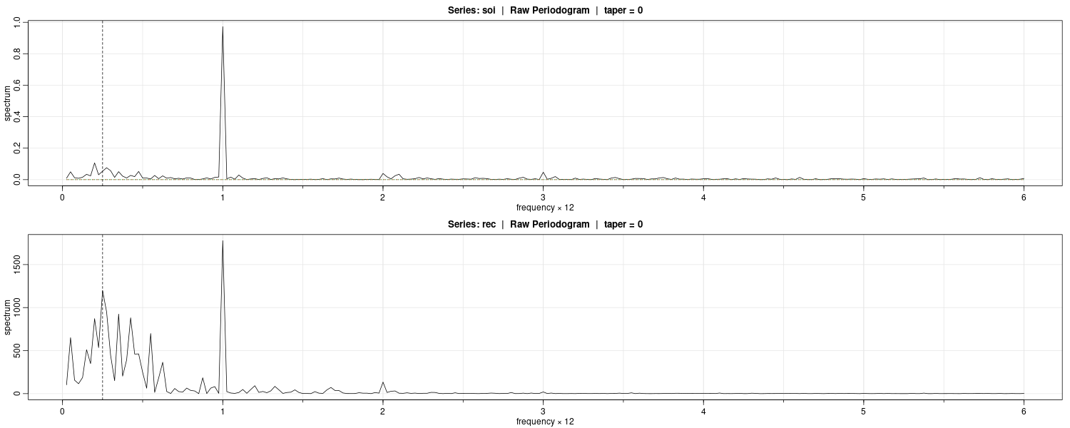
Nonparametric Spectral Estimation
We introduce a frequency band \(\mathcal{B}\), of \(L << n\) contiguous fundamental frequencies, centered around frequency \(\omega_{j} = \frac{j}{n}\). This frequency is chosen close to a frequency of interest \(\omega\).
For frequencies of the form:
\[\begin{aligned} \mathcal{B} &= \{\omega^{*}: \omega_{j} - \frac{m}{n} \leq \omega^{*} \leq \omega_{j} + \frac{m}{n}\} \end{aligned}\] \[\begin{aligned} \omega^{*} &= \omega_{j}+ \frac{k}{n}\\ k &= -m, \cdots, 0, \cdots, m\\ L &= 2m + 1 \end{aligned}\]Such that the spectral values in the interval \(\mathcal{B}\):
\[\begin{aligned} f(\omega_{j} + \frac{k}{n}) \end{aligned}\] \[\begin{aligned} k &= -m, \cdots, 0, \cdots, m \end{aligned}\]Are approximately equal to \(f(\omega)\).
This structure can be realized for large sample sizes.
We now define an averaged (or smoothed) periodogram as the average of the periodogram values over the band \(\mathcal{B}\):
\[\begin{aligned} \bar{f}(\omega) &= \frac{1}{L}\sum_{k=-m}^{m}I(\omega_{j} + \frac{k}{n}) \end{aligned}\]The bandwidth is defined as:
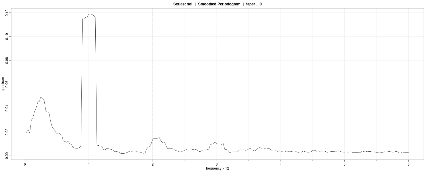
\[\begin{aligned} B = \frac{L}{n} \end{aligned}\]Example: Averaged Periodogram for SOI and Recruitment
Let’s try to show a smoothed periodogram using the SOI and Rec dataset. Using \(L = 9\) (via trial and error) which result in:
\[\begin{aligned} L &= 2m + 1 \end{aligned}\] \[\begin{aligned} m &= \frac{L - 1}{2}\\ &= 4 \end{aligned}\]In R using Daniell kernel:
soi.ave <- mvspec(
  soi,
  kernel("daniell", 4),
  log = "no"
)
abline(
  v = c(.25, 1, 2, 3),
  lty = 2
)
Contrast this with the periodogram:
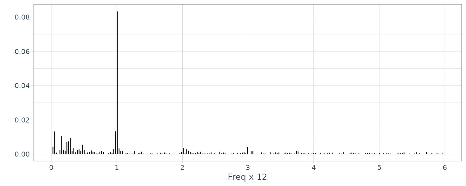
n <- nrow(soi)
soi$P <- 4 / n *
  Mod(fft(soi$value) / sqrt(n))^2
soi$freq <- 0:(n-1) / n

soi |>
  slice(2:(n() / 2)) |>
  ggplot(aes(x = freq, y = P)) +
  geom_segment(
    aes(
      x = freq,
      xend = freq,
      y = 0,
      yend = P
    )
  ) +
  ylab("") +
  theme_tq()
Note that mvspec shows the frequency in years rather than months.
The smoothed spectra shown provide a sensible compromise between the noisy version, and a more heavily smoothed spectrum, which might lose some of the peaks.
An undesirable effect of averaging can be noticed at the yearly cycle, \(\omega = 1\Delta\), where \(\Delta = \frac{1}{12}\) and the narrow band peaks that appeared in the periodograms have been flattened and spread out to nearby frequencies.
We also notice, and have marked, the appearance of harmonics of the yearly cycle, that is, frequencies of the form \(\omega = k\Delta\) for k = 1, 2, ….
The bandwidth:
> soi.ave$n.used
[1] 480

> soi.ave$bandwidth
[1] 0.225
Is calculated by adjusting it in terms of cycle per years from months (480 months via padding):
\[\begin{aligned} B &= \frac{L}{n}\\ &= \frac{9}{480}\\ &= 0.225\\ &= \frac{9}{480} \times 12 \end{aligned}\]Rather than using simple averaging, we can employ weighted averaging such that the weights decrease as distance from the center increase. An example would be the modified Daniell kernel. We will use it in the example below:
Example: Smoothed Periodogram for SOI and Recruitment
We will estimate the spectra of the SOI series using a modified Daniell kernel twice, with \(m=3\) (this is done by c(3, 3) in R) both times.
k <- kernel(
  "modified.daniell",
  c(3, 3)
)
soi.smo <- mvspec(
  soi,
  kernel = k,
  taper = .1,
  log = "no"
)
abline(v = c(.25, 1), lty = 2) 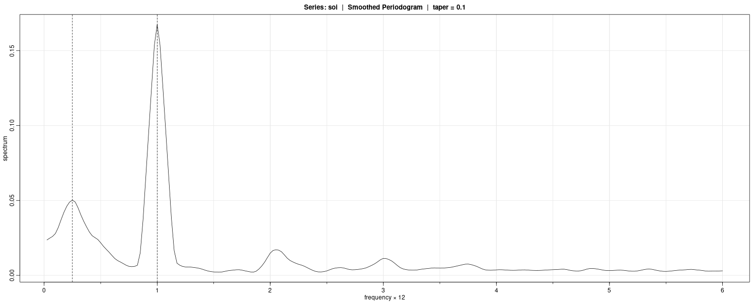
Tapering is done on the upper and lower 10% of the data.
Tapering
Suppose \(x_{t}\) is a zero-mean, stationary process with spectral density \(f_{x}(\omega)\). If we replace the original series by the taper series \(y_{t\)}:
\[\begin{aligned} y_{t} &= h_{t}x_{t} \end{aligned}\] \[\begin{aligned} t = 1, 2, \cdots, n \end{aligned}\]Taking the DFT of \(y_{t}\):
\[\begin{aligned} d_{y}(\omega_{j}) &= \frac{1}{\sqrt{n}}\sum_{t=1}^{n}h_{t}x_{t}e^{-2\pi i \omega \omega_{j}t} \end{aligned}\]Taking expection:
\[\begin{aligned} E[|d_{y}(\omega_{j})|^{2}] &= \int_{-\frac{1}{2}}^{\frac{1}{2}}|H_{n}(\omega_{j} - \omega)|^{2}f_{x}(\omega)\ d\omega\\ &= \int_{-\frac{1}{2}}^{\frac{1}{2}}W_{n}(\omega_{j} - \omega)f_{x}(\omega)\ d\omega\\ \end{aligned}\]Where:
\[\begin{aligned} W_{n}(\omega) &= |H_{n}(\omega)|^{2}\\ H_{n}(\omega) &= \frac{1}{\sqrt{n}}\sum_{t=1}^{n}h_{t}e^{-2\pi i \omega t} \end{aligned}\]| \(W_{n}(\omega)\) is called a spectral window. In the case that \(h_{t}=1\), $$ | d_{y(\omega_{j}) | ^{2}}$$ is just the periodogram of the data and the windown is: |
Tapers generally have a shape that enhances the center of the data relative to the extremities, such as a cosine bell of the form:
\[\begin{aligned} h_{t} &= 0.5\Big[1 + \mathrm{cos}\Big(\frac{2\pi(t - \frac{n+1}{2})}{n}\Big)\Big] \end{aligned}\]Untapered window contains considerable ripples over the band and outside the band. The ripples outside the band are called sidelobes and tend to introduce frequencies from outside the interval that may contaminate the desired spectral estimate within the band.
Parametric Spectral Estimation
The methods of the previous section lead to what is generally referred to as non-parametric spectral estimators because no assumption is made about the parametric form of the spectral density.
However, we know the spectral density of an ARMA process:
\[\begin{aligned} f_{x}(\omega) &= \sigma_{w}^{2}\frac{|\theta(e^{-2\pi i \omega})|^{2}}{|\phi(\phi(e^{-2\pi i \omega}))|^{2}} \end{aligned}\]For convenience, a parametric spectral estimator is obtained by fitting an AR(p) to the data, where the order p is determined by one of the model selection criteria, such as AIC, AICc, and BIC. Parametric autoregressive spectral estimators will often have superior resolution in problems when several closely spaced narrow spectral peaks are present and are preferred by engineers for a broad variety of problems.
If \(\hat{\phi}_{1}, \hat{\phi}_{2}, \cdots, \hat{\phi}_{p}, \hat{\sigma}_{w}^{2}\) are the estimates from an AR(p) fit to \(x_{t}\), a parametric spectral estimate of \(f_{x}(\omega)\) is attained by substituting these estimates into:
\[\begin{aligned} \hat{f}_{x}(\omega) &= \frac{\hat{\sigma}_{w}^{2}}{|\hat{\phi}(e^{-2\pi i \omega})|^{2}} \end{aligned}\] \[\begin{aligned} \hat{\phi}(z) &= 1 - \hat{\phi}_{1}z - \hat{\phi}_{2}z^{2} - \cdots - \hat{\phi}_{p}z^{p} \end{aligned}\]To do this in R:
spaic <- spec.ar(as.ts(soi), log = "no")
abline(v = frequency(soi) * 1 / 52, lty = 3) 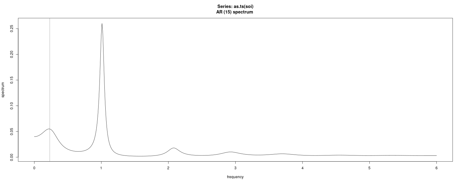
Multiple Series and Cross-Spectra
The notion of analyzing frequency fluctuations using classical statistical ideas extends to the case in which there are several jointly stationary series, for example, \(x_{t}, y_{t}\). In this case, we can introduce the idea of a correlation indexed by frequency, called the coherence.
It can be shown that the covariance function:
\[\begin{aligned} \gamma_{xy}(h) &= E[(x_{t+h}- \mu_{x})(y_{t} - \mu_{y})] \end{aligned}\]Has the representation:
\[\begin{aligned} \gamma_{xy}(h) &= \int_{-\frac{1}{2}}^{\frac{1}{2}}f_{xy}(\omega)e^{2\pi i \omega h}\ d\omega \end{aligned}\]Where the cross-spectrum is defined as the Fourier transform:
\[\begin{aligned} f_{xy}(\omega) &= \sum_{h=-\infty}^{\infty}\gamma_{xy}(h)e^{-2\pi i \omega h} \end{aligned}\] \[\begin{aligned} h &= 0, \pm 1, \pm 2 \end{aligned}\] \[\begin{aligned} -\frac{1}{2} \leq \omega \leq \frac{1}{2} \end{aligned}\]Assuming that the cross-covariance function is absolutely summable, as was the case for the autocovariance.
An important example of the application of the cross-spectrum is to the problem of predicting an output series \(y_{t}\) from some input series \(x_{t}\) through a linear filter relation such as the three-point moving average considered below.
The cross-spectrum is generally a complex-valued function:
\[\begin{aligned} f_{xy}(\omega) &= c_{xy}(\omega) - i q_{xy}(\omega)\\ c_{xy}(\omega) &= \sum_{h=-\infty}^{\infty}\gamma_{xy}(h)\mathrm{cos}(2\pi\omega h)\\ q_{xy}(\omega) &= \sum_{h=-\infty}^{\infty}\gamma_{xy}(h)\mathrm{sin}(2\pi\omega h) \end{aligned}\]Are defined as the cospectrum and quadspectrum.
Because \(\gamma_{yx}(h) = \gamma_{xy}(-h)\):
\[\begin{aligned} f_{yx}(\omega) &= f_{xy}^{*}(\omega)\\ c_{yx}(\omega) &= c_{xy}(\omega)\\ q_{yx}(\omega) &= -q_{xy}(\omega) \end{aligned}\]A measure of the strength of such a relation is the squared coherence function, defined as:
\[\begin{aligned} \rho_{yx}^{2}(\omega) &= \frac{|f_{yx}(\omega)|^{2}}{f_{xx}(\omega)f_{yy}(\omega)} \end{aligned}\]Notice the similarity with the conventional squared correlation:
\[\begin{aligned} \rho_{yx}^{2} &= \frac{\sigma_{yx}^{2}}{\sigma_{x}^{2}\sigma_{y}^{2}} \end{aligned}\]Coherency is a tool for relating the common periodic behavior of two series. Coherency is a frequency based measure of the correlation between two series at a given frequency, and it measures the performance of the best linear filter relating the two series.
Spectral Representation of a Vector Stationary Process
If \(\boldsymbol{x}_{t}\) is a px1 stationary process with autocovariance:
\[\begin{aligned} \boldsymbol{\Gamma}(h) &= E[(\boldsymbol{x}_{t+h} - \boldsymbol{\mu})(\boldsymbol{x}_{t+h} - \boldsymbol{\mu})^{T}]\\ &=\{\gamma_{jk}(h)\} \end{aligned}\] \[\begin{aligned} \sum_{h=-\infty}^{\infty}|\gamma_{jk}(h)| &< \infty \end{aligned}\] \[\begin{aligned} \boldsymbol{x}_{t} &= \begin{bmatrix} x_{t1}\\ x_{t2}\\ \vdots\\ x_{tp} \end{bmatrix} \end{aligned}\]Then:
\[\begin{aligned} \boldsymbol{\Gamma}(h) &= \int_{-\frac{1}{2}}^{\frac{1}{2}}e^{2\pi i \omega h} \end{aligned}\] \[\begin{aligned} \boldsymbol{f}(\omega) &= \{f_{ij}(\omega)\}\\ \end{aligned}\] \[\begin{aligned} j, k &= 1, \cdots, p \end{aligned}\] \[\begin{aligned} h &= 0, \pm 1, \pm2, \cdots \end{aligned}\]And the inverse transform of the spectral density matrix:
\[\begin{aligned} \textbf{f}(\omega) &= \sum_{h=-\infty}^{\infty}\boldsymbol{\Gamma}(h)e^{-2\pi i \omega h} \end{aligned}\] \[\begin{aligned} -\frac{1}{2} \leq \omega \leq \frac{1}{2} \end{aligned}\]The spectracl matrix \(\textbf{f}(\omega)\) is Hermitian (conjugate and transpose):
\[\begin{aligned} \textbf{f}(\omega) &= f^{*}(\omega) \end{aligned}\]Example: Three-Point Moving Average
Consider a 3-piont moving average where \(x_{t}\) is a stationary input process with spectral density \(f_{xx}(\omega)\):
\[\begin{aligned} y_{t} = \frac{x_{t-1} + x_{t} + x_{t+1}}{3} \end{aligned}\]First the autocovariance function:
\[\begin{aligned} \gamma_{xy}(h) &= \mathrm{cov}(x_{t+h}, y_{t})\\ &= \frac{1}{3}E[x_{t+h}(x_{t-1} + x_{t} + x_{t+1})]\\ &= \frac{1}{3}\Big[\gamma_{xx}(h + 1) + \gamma_{xx}(h) + \gamma_{xx}(h - 1)\Big] \end{aligned}\]Recall that the autocovariance function has the representation:
\[\begin{aligned} \gamma(h) &= \int_{-\frac{1}{2}}^{\frac{1}{2}}e^{2\pi i \omega h}f(\omega)\ d\omega \end{aligned}\]Hence:
\[\begin{aligned} \gamma_{xy}(h) &= \frac{1}{3}\Big[\gamma_{xx}(h + 1) + \gamma_{xx}(h) + \gamma_{xx}(h - 1)\Big]\\ &= \frac{1}{3}\int_{-\frac{1}{2}}^{\frac{1}{2}}(e^{2\pi i \omega(h + 1)} + e^{2\pi i \omega(h)} + e^{2\pi i \omega(h - 1)})f_{xx}(\omega)\ d\omega\\ &= \frac{1}{3}\int_{-\frac{1}{2}}^{\frac{1}{2}}(e^{2\pi i \omega} + 1 + e^{-2\pi i \omega})e^{2\pi i \omega h}f_{xx}(\omega)\ d\omega\\ &= \frac{1}{3}\int_{-\frac{1}{2}}^{\frac{1}{2}}[1 + 2\mathrm{cos}(2\pi\omega)]f_{xx}(\omega)e^{2\pi i \omega h}\ d\omega \end{aligned}\]Using the uniqueness of the Fourier transform, we conclude the spectral representation of \(\gamma_{xy}\) is:
\[\begin{aligned} f_{xy}(\omega) &= \frac{1}{3}[1 + 2\mathrm{cos}(2\pi\omega)]f_{xx}(\omega) \end{aligned}\]We will show later in the Linear Filter section that:
\[\begin{aligned} f_{y}(\omega) &= |A(\omega)|^{2}f_{x}(\omega)\\ A(\omega) &= \sum_{j=-\infty}^{\infty}a_{j}e^{-2\pi i \omega j} \end{aligned}\]Thus:
\[\begin{aligned} f_{yy}(\omega) &= \Big(\frac{1}{3}\Big)^{2}|e^{2\pi i \omega} + 1 + e^{-2\pi i \omega}|^{2}f_{xx}(\omega)\\ &= \frac{1}{9}\Big(1 + 2\mathrm{cos}(2\pi\omega)\Big)^{2}f_{xx}(\omega) \end{aligned}\]Finally getting the squared coherence:
\[\begin{aligned} \rho_{yx}^{2}(\omega) &= \frac{\Big|\frac{1}{3}[1 + 2\mathrm{cos}(2\pi\omega)]f_{xx}(\omega)\Big|^{2}}{f_{xx}(\omega)\times\frac{1}{9}\Big(1 + 2\mathrm{cos}(2\pi \omega))^{2}f_{xx}(\omega)}\\ &= 1 \end{aligned}\]That is, the squared coherence between \(x_{t}\) and \(y_{t}\) is unity over all frequencies. This is a characteristic inherited by more general linear filters. However, if some noise is added to the three-point moving average, the coherence is not unity.
Linear Filters
In this section, we explore that notion further by showing how linear filters can be used to extract signals from a time series. These filters modify the spectral characteristics of a time series in a predictable way.
Recall that:
\[\begin{aligned} y_{t} &= \sum_{j=-\infty}^{\infty}a_{j}x_{t-j} \end{aligned}\] \[\begin{aligned} \sum_{j=-\infty}^{\infty}|a_{j}| &< \infty \end{aligned}\] \[\begin{aligned} f_{yy}(\omega) &= |A_{yx}(\omega)|^{2}f_{xx}(\omega)\\ A_{yx(\omega)} &= \sum_{j=-\infty}^{\infty}a_{j}e^{-2\pi i \omega j} \end{aligned}\]\(A_{yx}(\omega)\) is known as the frequency response function. This result shows that the filtering effect can be characterized as a frequency-by-frequency multiplication by the squared magnitude of the frequency response function.
First Difference and Moving Average Filters
We consider two filters in this example.
The first difference filter:
\[\begin{aligned} y_{t} &= \nabla x_{t}\\ &= x_{t} - x_{t-1} \end{aligned}\]And the annual symmetric moving average filter (which is a modified Daniell kernel with m = 6):
\[\begin{aligned} y_{t} &= \frac{1}{24}(x_{t-6} + x_{t+6}) + \frac{1}{12}\sum_{r=-5}^{5}x_{t-r} \end{aligned}\]In general, differencing is an example of a high-pass filter because it retains or passes the higher frequencies, whereas the moving average is a low-pass filter because it passes the lower or slower frequencies.
Recall that:
\[\begin{aligned} A(\omega) &= \sum_{j=-\infty}^{\infty}a_{j}e^{-2\pi i \omega j} \end{aligned}\]First difference can be written as:
\[\begin{aligned} a_{0} &= 1\\ a_{1} &= -1\\ A_{yx}(\omega) &= 1 - e^{-2\pi i \omega} \end{aligned}\] \[\begin{aligned} |A_{yx}(\omega)|^{2} &= (1 - e^{-2\pi i \omega})(1 - e^{-2\pi i \omega})\\ &= 2[1 - \mathrm{cos(2\pi \omega)}] \end{aligned}\]Plotting the squared frequency response function:
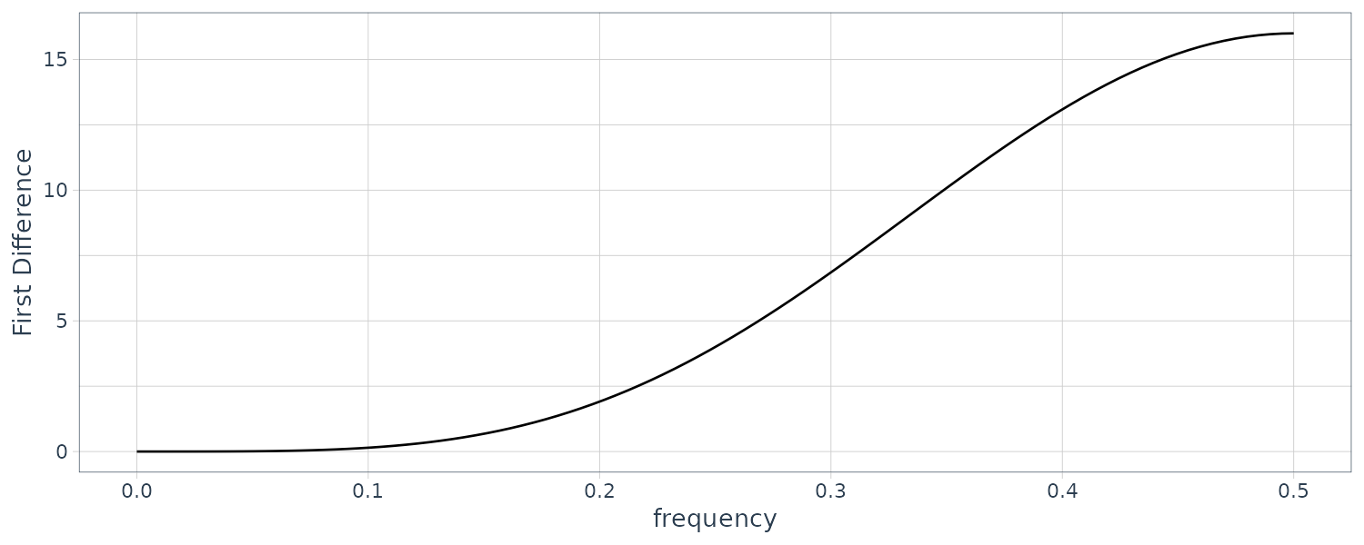
The first difference filter will attenuate the lower frequencies and enhance the higher frequencies because the multiplier of the spectrum, \(\mid A_{yw}(\omega)\mid^{2}\), is large for the higher frequencies and small for the lower frequencies.
For the centered 12-month moving average:
\[\begin{aligned} a_{-6} &= \frac{1}{24}\\ a_{6} &= \frac{1}{24}\\ a_{k} &= \frac{1}{12}\\ \end{aligned}\] \[\begin{aligned} -5 \leq k \leq 5 \end{aligned}\]This result in:
\[\begin{aligned} A_{yw}(\omega) &= \frac{1}{24}e^{2\pi i \omega 6} + \frac{1}{24}e^{-2\pi i \omega 6} + \frac{1}{12}\sum_{j=-5}^{-1}e^{-2\pi i \omega j} + \frac{1}{12}e^{0} + \frac{1}{12}\sum_{j=1}^{5}e^{-2\pi i \omega j}\\ &= \frac{1}{12}\Big[1 + \mathrm{cos}(12\pi\omega) + 2\sum_{k=1}^{5}\mathrm{cos}(2\pi\omega k)\Big] \end{aligned}\]Plotting the squared frequency response in R:
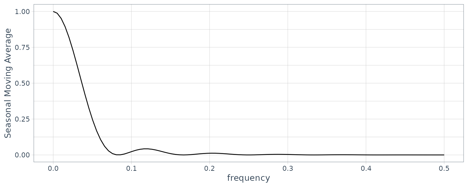
We can expect this filter to cut most of the frequency content above .05 cycles per point, and nearly all of the frequency content above \(\frac{1}{12} \approx 0.083\). In particular, this drives down the yearly components with periods of 12 months and enhances the El Niño frequency, which is somewhat lower.
Cross Spectrum
We can show that the cross-spectrum satisfies:
\[\begin{aligned} f_{yx}(\omega) &= A_{yx}(\omega)f_{xx}(\omega) \end{aligned}\] \[\begin{aligned} A_{yx}(\omega) &= \frac{f_{yx}(\omega)}{f_{xx}(\omega)}\\ &= \frac{c_{yx}(\omega)}{f_{xx}(\omega)} - i \frac{q_{yx}(\omega)}{f_{xx}(\omega)} \end{aligned}\]Note the difference between that and:
\[\begin{aligned} f_{yy}(\omega) &= |A_{yx}|^{2}(\omega)f_{xx}(\omega)\\ \end{aligned}\]We may rewrite in polar form:
\[\begin{aligned} A_{yx}(\omega) &= |A_{yx}(\omega)|e^{-i \phi_{yx}(\omega)}\\ |A_{yx}(\omega)| &= \frac{\sqrt{c_{yx}^{2}(\omega) + q_{yx}^{2}(\omega)}}{f_{xx}(\omega)}\\ \phi_{yx}(\omega) &= \mathrm{tan}^{-1}\Big(-\frac{q_{xx}(\omega)}{c_{yx}(\omega)}\Big) \end{aligned}\]A simple interpretation of the phase of a linear filter is that it exhibits time delays as a function of frequency in the same way as the spectrum represents the variance as a function of frequency.
Example: Simple Delaying Filter
Consider the simple delaying filter where the series gets replaced by a version, amplified by multiplying by A and delayed by D points:
\[\begin{aligned} y_{t} &= A x_{t-D} \end{aligned}\] \[\begin{aligned} A_{yw} &= \sum_{j=-\infty}^{\infty}a_{j}e^{-2\pi i \omega j}\\ &= Ae^{-2\pi i \omega D} \end{aligned}\] \[\begin{aligned} f_{yx}(\omega) &= A_{yw}f_{xx}(\omega)\\ &= Ae^{-2\pi i \omega D}f_{xx}(\omega) \end{aligned}\]Recall that:
\[\begin{aligned} A_{yw} &= |A_{yx}(\omega)|e^{-i \phi_{yx}(\omega)} \end{aligned}\]Hence:
\[\begin{aligned} |A_{yx}(\omega)| &= A\\ \phi_{yx}(\omega) &= -2\pi \omega D \end{aligned}\]Applying a simple time delay causes phase delays that depend on the frequency of the periodic component being delayed.
For example:
\[\begin{aligned} x_{t} &= \mathrm{cos}(2\pi\omega t)\\ y_{t} &= Ax_{t-D}\\ &= \mathrm{cos}(2\pi\omega(t- D))\\ &= A\mathrm{cos}(2\pi\omega t - 2\pi\omega D) \end{aligned}\]Thus, the output series, \(y_{t}\), has the same period as the input series, xt , but the amplitude of the output has increased by a factor of \(\mid A \mid\) and the phase has been changed by a factor of \(-2\pi\omega D\).
Example: Difference and Moving Average Filters
The case for the moving average is easy because \(A_{yx}(\omega)\) is purely real. So, the amplitude is just \(\mid A_{yx}(\omega)\mid\) and the phase is \(\phi_{yx}(\omega) = 0\). In general, symmetric \((a_{j} = a_{-j})\) filters have zero phase.
The first difference, however, changes this. In this case, the squared amplitude is:
\[\begin{aligned} |A_{yx}(\omega)|^{2} &= (1 - e^{-2\pi i \omega})(1 - e^{2\pi i \omega})\\ &= 2[1 - \mathrm{cos(2\pi \omega)}] \end{aligned}\]To compute the phase:
\[\begin{aligned} A_{yx}(\omega) &= 1 - e^{-2\pi i \omega}\\ &= e^{-i\pi\omega}(e^{i\pi\omega} - e^{-i\pi\omega})\\ &= 2i e^{-i\pi\omega}\mathrm{sin}(\pi\omega)\\ &= 2\mathrm{sin}^{2}(\pi\omega) + 2i\mathrm{cos}(\pi\omega)\mathrm{sin}(\pi\omega)\\ &= \frac{c_{yx}(\omega)}{f_{xx}(\omega)} - i \frac{q_{yx}(\omega)}{f_{xx}(\omega)} \end{aligned}\]So:
\[\begin{aligned} \phi_{yx}(\omega) &= \mathrm{tan}^{-1}\Big(-\frac{q_{yx}(\omega)}{c_{yx}(\omega)}\Big)\\ &= \mathrm{tan}^{-1}\Big(-\frac{2\mathrm{cos}(\pi\omega)\mathrm{sin}(\pi\omega)}{2\mathrm{sin}^{2}(\pi\omega)}\Big)\\ &= \mathrm{tan}^{-1}\Big(-\frac{\mathrm{cos}(\pi\omega)}{\mathrm{sin}(\pi\omega)}\Big) \end{aligned}\]Note that:
\[\begin{aligned} \mathrm{cos}(\pi\omega) &= \mathrm{sin}\Big(-\pi\omega + \frac{\pi}{2}\Big)\\ \mathrm{sin}(\pi\omega) &= \mathrm{cos}\Big(-\pi\omega + \frac{\pi}{2}\Big)\\ \end{aligned}\]Thus:
\[\begin{aligned} \phi_{yx}(\omega) &= \mathrm{tan}^{-1}\Bigg(\frac{\mathrm{sin}(-\pi\omega + \frac{\pi}{2})}{\mathrm{cos}(-\pi\omega + \frac{\pi}{2})}\Bigg)\\ &= \mathrm{tan}^{-1}\mathrm{tan}\Big(-\pi\omega + \frac{\pi}{2}\Big)\\ &= -\pi\omega + \frac{\pi}{2} \end{aligned}\]Lagged Regression Models
One of the intriguing possibilities offered by the coherence analysis of the relation between the SOI and Recruitment series would be extending classical regression to the analysis of lagged regression models of the form:
\[\begin{aligned} y_{t} &= \sum_{r=-\infty}^{\infty}\beta_{r}x_{t-r} + v_{t} \end{aligned}\]We assume that the inputs and outputs have zero means and are jointly stationary with the 2 x 1 vector process \((x_{t}, y_{t})\) having a spectral matrix of the form:
\[\begin{aligned} f(\omega) &= \begin{bmatrix} f_{xx}(\omega) & f_{xy}(\omega)\\ f_{yx}(\omega) & f_{yy}(\omega) \end{bmatrix} \end{aligned}\]We assume all autocovariance functions satisfy the absolute summability conditions.
Minimizing the MSE:
\[\begin{aligned} MSE = E\Big[y_{t} - \sum_{r=-\infty}^{\infty}\beta_{r}x_{t-r}\Big]^{2} \end{aligned}\]Leads to the orthogonality conditions:
\[\begin{aligned} E\Big[\Big(y_{t} - \sum_{r=-\infty}^{\infty}\beta_{r}x_{t-r}\Big)x_{t-s}\Big] &= 0 \end{aligned}\] \[\begin{aligned} s &= 0, \pm 1, \pm 2, \cdots \end{aligned}\]Taking expectations inside leads to the normal equations:
\[\begin{aligned} E[y_{t}x_{t-s} - \sum_{r=-\infty}^{\infty}\beta_{r}x_{t-r}x_{t-s}] &= 0\\ E[y_{t}x_{t-s}] - \sum_{r=-\infty}^{\infty}\beta_{r}E[x_{t-r}x_{t-s}] &= 0 \end{aligned}\] \[\begin{aligned} \sum_{r=-\infty}^{\infty}\beta_{r}\gamma_{xx}(s-r) &= \gamma_{yx}(s) \end{aligned}\]Using spectral representation:
\[\begin{aligned} \int_{-\frac{1}{2}}^{\frac{1}{2}}\sum_{r=-\infty}^{\infty}\beta_{r}e^{2\pi i \omega(s-r)}f_{xx}(\omega)\ d\omega &= \int_{-\frac{1}{2}}{\frac{1}{2}}e^{2\pi i \omega s}f_{xy}(\omega)\ d\omega\\ \int_{-\frac{1}{2}}^{\frac{1}{2}}e^{2\pi i \omega s}B(\omega)f_{xx}(\omega)\ d\omega &= \int_{-\frac{1}{2}}{\frac{1}{2}}e^{2\pi i \omega s}f_{xy}(\omega)\ d\omega \end{aligned}\]Where \(B(\omega)\) is the Fourier transform of the regression coefficients:
\[\begin{aligned} B(\omega) &= \sum_{r=-\infty}^{\infty}\beta_{r}e^{-2\pi i \omega r} \end{aligned}\]We might write the system of equations in the frequency domain, using the uniqueness of the Fourier transform:
\[\begin{aligned} B(\omega)f_{xx}(\omega) &= f_{yx}(\omega) \end{aligned}\]Taking the estimator for the Fourier transform of the regression coefficients evaluated at some fundamental frequiencies:
\[\begin{aligned} \hat{B}(\omega_{k}) &= \frac{\hat{f}_{yx}(\omega_{k})}{\hat{f}_{xx}(\omega_{k})}\\ \omega_{k} &= \frac{k}{M}\\ M &<< n \end{aligned}\]The inverse transform of the function \(\hat{B}(\omega)\):
\[\begin{aligned} \hat{\beta}_{t} &= M^{-1}\sum_{k=0}^{M-1}\hat{B}(\omega_{k})e^{2\pi i \omega_{k}t}\\ t &= 0, \pm 1, \cdots \pm\Big(\frac{M}{2-1}\Big) \end{aligned}\]Example: Lagged Regression for SOI and Recruitment
The high coherence between the SOI and Recruitment series noted suggests a lagged regression relation between the two series. The model is:
\[\begin{aligned} y_{t} &= \sum_{r=-\infty}^{\infty}a_{r}x_{t-r} + w_{t}\\ x_{t} &= \sum_{r=-\infty}^{\infty}b_{r}y_{t-r} + v_{t} \end{aligned}\]Even though there is no plausible environmental explanation for the second of these two models, displaying both possibilities helps to settle on a parsimonious transfer function model.
Signal Extraction and Optimum Filtering
Assuming that:
\[\begin{aligned} y_{t} &= \sum_{r=-\infty}^{\infty}\beta_{r}x_{t-r} + v_{t} \end{aligned}\]Assuming that \(\beta\) are known and \(x_{t}\) are unknown. In this case, we are interested in an estimator for the signal \(x_{t}\) of the form:
\[\begin{aligned} \hat{x}_{t} &= \sum_{r=-\infty}^{\infty}a_{r}y_{t-r} \end{aligned}\]Often, the special case is where the relation reduces to the simple signal plus noise model:
\[\begin{aligned} y_{t} = x_{t} + v_{t} \end{aligned}\]In general, we seek to find the set of filter coefficients \(a_{t}\) that minimize the MSE:
\[\begin{aligned} MSE = E\Big[x_{t} - \sum_{r=-\infty}^{\infty}a_{r}y_{t-r}\Big]^{2} \end{aligned}\]Applying the orthogonality principle:
\[\begin{aligned} E\Big[\Big(x_{t} - \sum_{r=-\infty}^{\infty}a_{r}y_{t-r}\Big)y_{t-s}\Big] = 0 \end{aligned}\] \[\begin{aligned} s &= 0, \pm 1, \pm 2, \cdots \end{aligned}\] \[\begin{aligned} \sum_{r=-\infty}^{\infty}a_{r}\gamma_{yy}(s - r) = \gamma_{xy}(s) \end{aligned}\]Substituting the spectral representations for the autocovariance functions into the above and identifying the spectral densities through the uniqueness of the Fourier transform produces:
\[\begin{aligned} A(\omega)f_{yy}(\omega) = f_{xy}(\omega) \end{aligned}\]The Fourier transform pair for \(A(\omega)\) and \(B(\omega)\):
\[\begin{aligned} A(\omega) &= \sum_{r=-\infty}^{\infty}a_{r} B(\omega) &= \sum_{r=-\infty}^{\infty}\beta_{r} \end{aligned}\]A special consequence of the model:
\[\begin{aligned} f_{xy}(\omega) &= B^{*}(\omega)f_{xx}(\omega)\\ f_{yy}(\omega) &= |B(\omega)|^{2}f_{xx}(\omega) + f_{vv}(\omega) \end{aligned}\]Implying that the optimal filter would be Fourier transform of:
\[\begin{aligned} A(\omega) &= \frac{B^{*}(\omega)}{\Big(|B(\omega)|^{2} + \frac{f_{vv}(\omega)}{f_{xx}(\omega)}\Big)} \end{aligned}\]The second term n the denominator is just the inverse of the signal to noise ratio:
\[\begin{aligned} \text{SNR}(\omega) &= \frac{f_{xx}(\omega)}{f_{vv}(\omega)} \end{aligned}\]It is possible to specify the signal-to-noise ratio a priori. If the signal-to-noise ratio is known, the optimal filter can be computed by the inverse transform of the function \(A(\omega)\). It is more likely that the inverse transform will be intractable and a finite filter approximation like that used in the previous section can be applied to the data. In this case, we will have the below as the estimated filter function:
\[\begin{aligned} a_{t}^{M} &= M^{-1}\sum_{k=0}^{M-1}A(\omega_{k})e^{2\pi i \omega_{k}t} \end{aligned}\]Using the tapered filter where \(h_{t}\) is the cosine taper:
\[\begin{aligned} \tilde{a}_{t} &= h_{t}a_{t} \end{aligned}\]The squared frequency response of the resulting filter:
\[\begin{aligned} \tilde{A}(\omega) &= \sum_{t=-\infty}^{\infty}a_{t}h_{t}e^{-2\pi i \omega t} \end{aligned}\]Example: Estimating the El Niño Signal via Optimal Filters
Looking at the spectrum of the SOI series:
We note that essentially two components have power, the El Niño frequency of about .02 cycles per month (the four-year cycle) and a yearly frequency of about .08 cycles per month (the annual cycle). We assume, for this example, that we wish to preserve the lower frequency as signal and to eliminate the higher order frequencies, and in particular, the annual cycle. In this case, we assume the simple signal plus noise model:
\[\begin{aligned} y_{t} &= x_{t} + v_{t} \end{aligned}\]Where there is no convolving function \(\beta_{t}\). Furthermore, the signal-to-noise ratio is assumed to be high to about .06 cycles per month and zero thereafter.
The optimal frequency response was assumed to be unity to .05 cycles per point and then to decay linearly to zero in several steps.
This can be done in R using SigExtract:
SigExtract(as.ts(soi), L = 9, M = 64, max.freq = 0.05) The filters we have discussed here are all symmetric two-sided filters, because the designed frequency response functions were purely real. Alternatively, we may design recursive filters to produce a desired response. An example of a recursive filter is one that replaces the input \(x_{t}\) by the filtered output:
\[\begin{aligned} y_{t} &= \sum_{k=1}^{p}\phi_{k}y_{t-k} + x_{t} - \sum_{k}^{1}\theta_{k}x_{t-l} \end{aligned}\]Note the similarity between the above equation and the ARMA(p, q) model, in which the white noise component is replaced by the input.
Using the property:
\[\begin{aligned} f_{y}(\omega) &= |A(\omega)|^{2}f_{x}(\omega)\\ &= \frac{|\theta(e^{-2\pi i \omega})|^{2}}{|\phi(e^{-2\pi i \omega})|^{2}}f_{x}(\omega) \end{aligned}\]Where:
\[\begin{aligned} \phi(e^{-2\pi i \omega}) &= 1 - \sum_{k=1}^{p}\phi_{k}e^{-2\pi i k \omega}\\ \theta(e^{-2\pi i \omega}) &= 1 - \sum_{k=1}^{q}\theta_{k}e^{-2\pi i k \omega} \end{aligned}\]Recursive filters such as those given above distort the phases of arriving frequencies.
