In this post, we will continue with Shumway H. (2017) Time Series Analysis, focusing on State Space Models. y

Introduction

A very general model that subsumes a whole class of special cases of interest in much the same way that linear regression does is the state-space model or the dynamic linear model. The model arose in the space tracking setting, where the state equation defines the motion equations for the position or state of a spacecraft with location \(x_{t}\) and the data \(y_{t}\) reflect information that can be observed from a tracking device such as velocity and azimuth.

In general, the state space model is characterized by two principles. First, there is a hidden or latent process \(x_{t}\) called the state process. The state process is assumed to be a Markov process; this means that the future \(\{x_{s} ; s > t\}\), and past \(\{x_{s} ; s < t\}\), are independent conditional on the present, \(x_{t}\). The second condition is that the observations, \(y_{t}\) are independent given the states \(x_{t}\). This means that the dependence among the observations is generated by states.

Linear Gaussian Model

The linear Gaussian state space model or dynamic linear model (DLM), in its basic form, employs an order one, p-dimensional vector autoregression as the state equation:

\[\begin{aligned} \textbf{x}_{t} &= \textbf{G}_{t}\textbf{x}_{t-1} + \boldsymbol{w}_{t} \end{aligned}\]

The \(\textbf{w}_{t}\) are p x 1 independent and identically distributed, zero-mean normal vectors with covariance matrix \(\textbf{W}_{t}\); we write this as:

\[\begin{aligned} \textbf{w}_{t} \sim N_{p}(\textbf{0}, \textbf{W}_{t}) \end{aligned}\]

In the DLM, we assume the process starts with a normal vector \(\textbf{x}_{0}\), such that:

\[\begin{aligned} \textbf{x}_{0} \sim N_{p}(\textbf{m}_{0}, \textbf{C}_{0}). \end{aligned}\]

We do not observe the state vector \(\textbf{x}_{t}\) directly, but only a linear transformed version of it with noise added, say:

\[\begin{aligned} \textbf{y}_{t} &= \textbf{F}_{t}\textbf{x}_{t} + \textbf{v}_{t} \end{aligned}\]

Where \(\textbf{F}_{t}\) is a q x p measurement or observation matrix and the above equation is called the observation equation. The observed data vector, \(\textbf{y}_{t}\), is q-dimensional, which can be larger than or smaller than p, the state dimension.

The additive observation noise is:

\[\begin{aligned} \textbf{v}_{t} ∼ N_{q}(\textbf{0}, \textbf{V}_{t}) \end{aligned}\]

In addition, we initially assume, for simplicity, \(\textbf{x}_{0}, \textbf{w}_{t}, \textbf{v}_{t}\) are uncorrelated; this assumption is not necessary.

In the ARMAX model which contains exogenous variables, or fixed inputs, may enter into the states or into the observations. In this case, we suppose we have an r x 1 vector of inputs \(\boldsymbol{\mu}_{t}\), and write the model as:

\[\begin{aligned} \textbf{x}_{t} &= \textbf{G}_{t} \textbf{x}_{t-1} + \Psi \boldsymbol{\mu}_{t} + \textbf{w}_{t}\\ \textbf{y}_{t} &= \textbf{F}_{t}\textbf{x}_{t} + \boldsymbol{\Gamma}_{t} \boldsymbol{\mu}_{t} + \textbf{v}_{t} \end{aligned}\]

Where \(\Psi\) is p x r and \(\boldsymbol{\Gamma}_{t}\) is q x r. Note either of these matrices may be the zero matrix.

Example: A Biomedical Example

Suppose we consider the problem of monitoring the level of several biomedical markers after a cancer patient undergoes a bone marrow transplant. The data are measurements made for 91 days on three variables:

• log(white blood count) [WBC]
• log(platelet) [PLT]
• hematocrit [HCT]

Denoted by:

\[\begin{aligned} \textbf{y}_{t} = \begin{bmatrix} y_{t1}\\ y_{t2}\\ y_{t3} \end{bmatrix} \end{aligned}\]

Approximately 40% of the values are missing, with missing values occurring primarily after the 35th day. The main objectives are to model the three variables using the state-space approach, and to estimate the missing values.

We model the three variables in terms of the state equation:

\[\begin{aligned} \begin{bmatrix} x_{t1}\\ x_{t2}\\ x_{t3} \end{bmatrix} &= \begin{bmatrix} \phi_{11} & \phi_{12} & \phi_{13}\\ \phi_{21} & \phi_{22} & \phi_{23}\\ \phi_{31} & \phi_{32} & \phi_{33} \end{bmatrix} \begin{bmatrix} x_{t-1,1}\\ x_{t-1, 2}\\ x_{t-1, 3} \end{bmatrix} + \begin{bmatrix} w_{t1}\\ w_{t2}\\ w_{t3} \end{bmatrix} \end{aligned}\]

And the observation equations:

\[\begin{aligned} \mathbf{y}_{t} &= \textbf{F}_{t}\mathbf{x}_{t} + \mathbf{v}_{t} \end{aligned}\]

Example: Global Warming

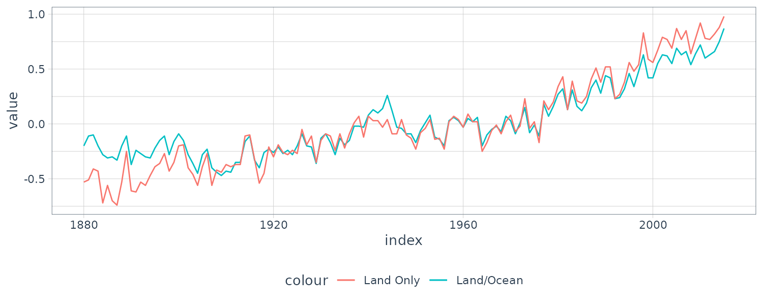
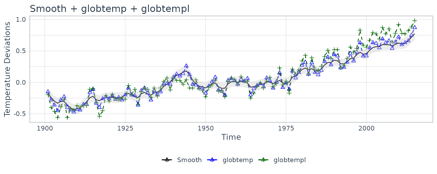
The above figure shows two different estimators for the global temperature series from 1880 to 2015. One is globtemp which contains the global mean land-ocean temperature index data. The second series, globtempl, are the surface air temperature index data using only meteorological station data.

Conceptually, both series should be measuring the same underlying climatic signal, and we may consider the problem of extracting this underlying signal.

We suppose both series are observing the same signal with different noises:

\[\begin{aligned} y_{t1} &= x_{t} + v_{t1}\\ y_{t2} &= x_{t} + v_{t2} \end{aligned}\] \[\begin{aligned} \begin{bmatrix} y_{t1}\\ y_{t2} \end{bmatrix} &= \begin{bmatrix} 1\\ 1 \end{bmatrix}x_{t} + \begin{bmatrix} v_{t1}\\ v_{t2} \end{bmatrix} \end{aligned}\]

And \(v_{ti}\) having the covariance matrix \(\textbf{V}_{t}\):

\[\begin{aligned} \textbf{V}_{t} &= \begin{bmatrix} V_{11} & V_{12}\\ V_{21} & V_{22} \end{bmatrix} \end{aligned}\]

We further assume and model \(x_{t}\) as a random walk with drift

\[\begin{aligned} x_{t} &= \delta + x_{t-1} + w_{t} \end{aligned}\]

And variance \(\textbf{W}_{t}\):

\[\begin{aligned} \textbf{W}_{t} = \text{var}(w_{t}) \end{aligned}\]

The introduction of the state-space approach as a tool for modeling data in the social and biological sciences requires model identification and parameter estimation because there is rarely a well-defined differential equation describing the state transition. The questions of general interest for the dynamic linear model (DLM) relate to estimating the unknown parameters contained in \(\textbf{G}_{t}, \Psi, \textbf{W}_{t}, \boldsymbol{\Gamma}_{t}, \textbf{F}_{t}, \textbf{V}_{t}\) that define the particular model, and estimating or forecasting values of the underlying unobserved process \(\textbf{x}_{t}\).

The advantages of the state-space formulation are in the ease with which we can treat various missing data configurations and in the incredible array of models that can be generated. The analogy between the observation matrix \(\textbf{F}_{t}\) and the design matrix in the usual regression and analysis of variance setting is a useful one. We can generate fixed and random effect structures that are either constant or vary over time simply by making appropriate choices for the matrix \(\textbf{F}_{t}\) and the transition structure \(\textbf{G}_{t}\).

Example: An AR(1) Process with Observational Noise

Consider a univariate state-space model where the observations are noisy:

\[\begin{aligned} y_{t} &= x_{t} + v_{t} \end{aligned}\]

And the signal/state is an AR(1) process:

\[\begin{aligned} x_{t} &= \phi x_{t-1} + w_{t} \end{aligned}\]

Where:

\[\begin{aligned} v_{t} &\sim N(0, \sigma_{v}^{2})\\ w_{t} &\sim N(0, \sigma_{w}^{2}) \end{aligned}\] \[\begin{aligned} x_{0} &\sim N\Big(0, \frac{\sigma_{w}^{2}}{1 - \phi^{2}}\Big) \end{aligned}\]

Recall if \(x_{t}\) is a stationary AR(1) process, the autocovariance function is:

\[\begin{aligned} \gamma_{x}(h) &= \frac{\sigma_{w}^{2}}{1 - \phi^{2}}\phi^{h} \end{aligned}\]

And the variance of \(y_{t}\):

\[\begin{aligned} \gamma_{y}(0) &= \textrm{var}(y_{t})\\ &= \textrm{var}(x_{t} + v_{})\\ &= \frac{\sigma_{w}^{2}}{1 - \phi^{2}} + \sigma_{v}^{2} \end{aligned}\]

And when \(h\geq 1\):

\[\begin{aligned} \gamma_{y}(h) &= \textrm{cov}(y_{t}, y_{t-h})\\ &= \textrm{cov}(x_{t} + v_{t}, x_{t-h} + v_{t-h})\\ &= \gamma_{x}(h) \end{aligned}\]

And the ACF:

\[\begin{aligned} \rho_{y}(h) &= \frac{\gamma_{y}(h)}{\gamma_{y}(0)}\\ &= \frac{\frac{\sigma_{w}^{2}}{1 - \phi^{2}}\phi^{h}}{\frac{\sigma_{w}^{2}}{1-\phi^{2}} + \sigma_{v}^{2}}\\ &= \frac{\phi^{h}}{1 + \frac{\sigma_{v}^{2}}{\sigma_{w}^{2}}(1 - \phi^{2})} \end{aligned}\]

It should be clear from the correlation structure that the observations, \(y_{t}\) , are not AR(1) unless \(\sigma_{v}^{2} = 0\). In addition, the autocorrelation structure of \(y_{t}\) is identical to the autocorrelation structure of an ARMA(1,1) process. Thus, the observations can also be written in an ARMA(1,1) form:

\[\begin{aligned} y_{t} &= \phi y_{t-1} + \theta e_{t-1} + e_{t} \end{aligned}\] \[\begin{aligned} e_{t} &\sim N(0, \sigma_{e}^{2}) \end{aligned}\]

Although an equivalence exists between stationary ARMA models and stationary state-space models, it is sometimes easier to work with one form than another. As previously mentioned, in the case of missing data, complex multivariate systems, mixed effects, and certain types of nonstationarity, it is easier to work in the framework of state-space models.

Filtering, Smoothing, and Forecasting

A primary aim of any analysis involving the state space model would be to produce estimators for the underlying unobserved signal \(\textbf{x}_{t}\), given the data \(\textbf{y}_{1:s}\).

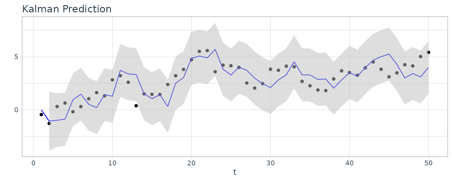
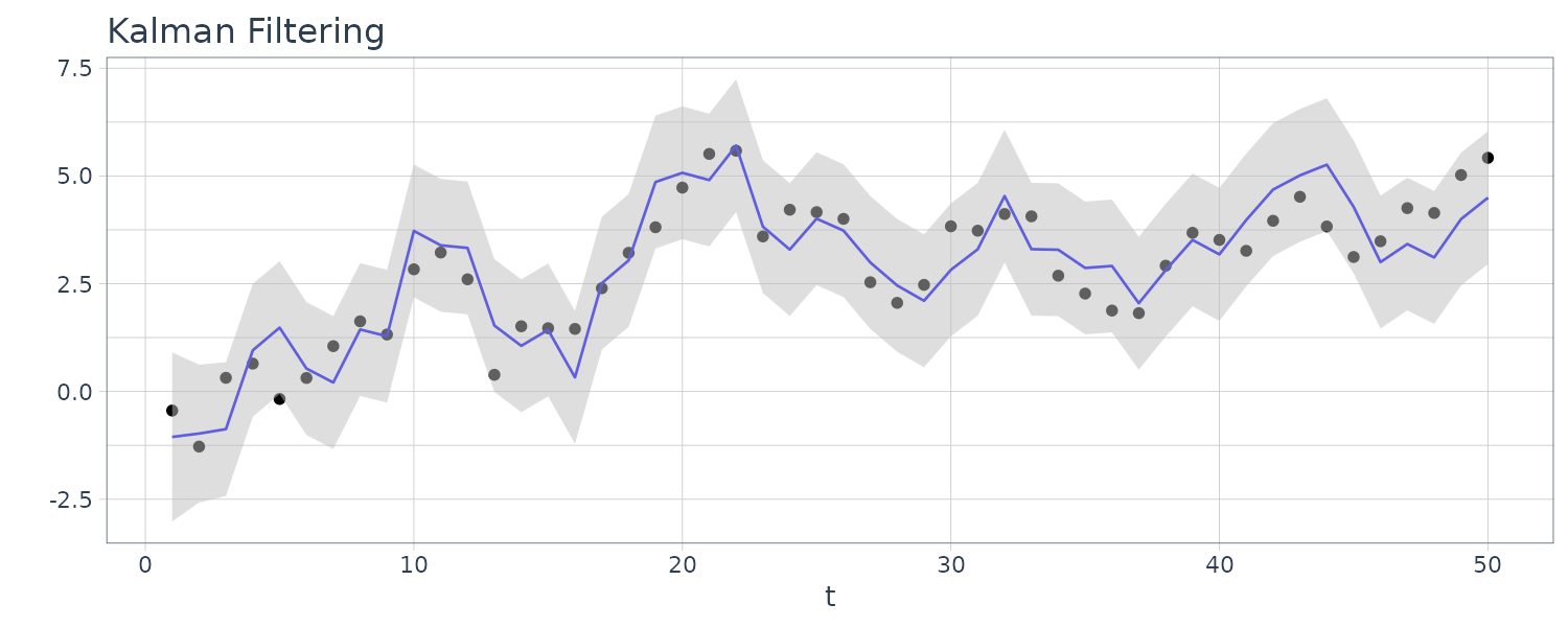
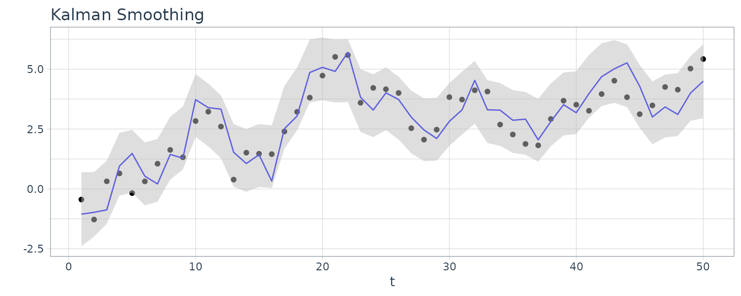
When \(s < t\), the problem is called forecasting or prediction. When \(s = t\), the problem is called filtering, and when \(s > t\), the problem is called smoothing. In addition to these estimates, we would also want to measure their precision. The solution to these problems is accomplished via the Kalman filter and smoother.

We will use the following definition:

\[\begin{aligned} \textbf{x}_{t}^{s} &= E[\textbf{x}_{t}|\textbf{y}_{1:s}] \end{aligned}\] \[\begin{aligned} \textbf{P}_{t1, t_{2}}^{s} &= E[(\textbf{x}_{t1} - \textbf{x}_{t1}^{s})(\textbf{x}_{t2} - \textbf{x}_{t2}^{s})^{T}] \end{aligned}\]

Kalman Filter

First, we present the Kalman filter, which gives the filtering and forecasting equations. The name filter comes from the fact that \(\textbf{x}_{t}^{t}\) is a linear filter of the observations \(\textbf{y}_{1:t}\); that is:

\[\begin{aligned} \textbf{x}_{t}^{t} &= \sum_{s=1}^{t}B_{s}\textbf{y}_{s} \end{aligned}\]

For suitably chosen p x q matrices \(B_{s}\). The advantage of the Kalman filter is that it specifies how to update the filter from \(\textbf{x}_{t−1}^{t-1}\) to \(\textbf{x}_{t}^{t}\) once a new observation \(\textbf{y}_{t}\) is obtained, without having to reprocess the entire data set \(\textbf{y}_{1:t}\).

With initial conditions:

\[\begin{aligned} \textbf{x}_{0}^{0} &= \textbf{m}_{0}\\ \textbf{P}_{0}^{0} &= \textbf{C}_{0} \end{aligned}\] \[\begin{aligned} t &= 1, \cdots, n \end{aligned}\]

The state-space model:

\[\begin{aligned} \textbf{x}_{t}^{t-1} &= \textbf{G}_{t} \textbf{x}_{t-1}^{t-1} + \Psi \textbf{u}_{t}\\ \textbf{P}_{t}^{t-1} &= \textbf{G}_{t} \textbf{P}_{t-1}^{t-1}\textbf{G}_{t}^{T} + \textbf{W}_{t} \end{aligned}\]

With:

\[\begin{aligned} \textbf{x}_{t}^{t} &= \textbf{x}_{t}^{t-1} + \textbf{K}_{t}(\textbf{y}_{t} - \textbf{F}_{t}\textbf{x}_{t}^{t-1} - \boldsymbol{\Gamma}_{t} \textbf{u}_{t})\\ \textbf{P}_{t}^{t} &= [\textbf{I} - \textbf{K}_{t}\textbf{F}_{t}]\textbf{P}_{t}^{t-1}\\ \textbf{K}_{t} &= \textbf{P}_{t}^{t-1}\textbf{F}_{t}^{T}[\textbf{F}_{t}\textbf{P}_{t}^{t-1}\textbf{F}_{t}^{T} + \textbf{V}_{t}]^{-1} \end{aligned}\]

\(\textbf{K}_{t}\) is known as the Kalman gain.

Important byproducts of the filter are the innovations:

\[\begin{aligned} \textbf{e}_{t} &= \textbf{y}_{t} - E[\textbf{y}_{t}|\textbf{y}_{1:t-1}]\\ &= \textbf{y}_{t} - \textbf{F}_{t}\textbf{x}_{t}^{t-1}- \boldsymbol{\Gamma}_{t} \textbf{u}_{t} \end{aligned}\]

And the covariance matrix:

\[\begin{aligned} \textbf{C}_{t} &\equiv \textrm{var}(\textbf{e}_{t})\\ &= \textrm{var}(\textbf{F}_{t}(\textbf{x}_{t} - \textbf{x}_{t}^{t-1}) + v_{t})\\ &= \textbf{F}_{t}\textbf{P}_{t}^{t-1}\textbf{F}_{t}^{T} + \textbf{V}_{t} \end{aligned}\]

Using these results we have that the joint conditional distribution of \(\textbf{x}_{t}\) and \(\textbf{e}_{t}\) given \(\textbf{y}_{1:t−1}\) is normal:

\[\begin{aligned} \begin{bmatrix} \textbf{x}_{t}\\ \textbf{e}_{t} \end{bmatrix} \Bigg| \textbf{y}_{1:t-1} &\sim N\Bigg( \begin{bmatrix} \textbf{x}_{t}^{t-1}\\ 0 \end{bmatrix}, \begin{bmatrix} \textbf{P}_{t}^{t-1} & \textbf{P}_{t}^{t-1}\textbf{F}_{t}^{T}\\ \textbf{F}_{t}\textbf{P}_{t}^{t-1} & \textbf{C}_{t} \end{bmatrix} \Bigg) \end{aligned}\]

Thus, we can write:

\[\begin{aligned} \textbf{x}_{t}^{t} &= E[\textbf{x}_{t}|\textbf{y}_{1:t}]\\ &= E[\textbf{x}_{t}|\textbf{y}_{1:t-1}, \textbf{e}_{t}]\\ &= \textbf{x}_{t}^{t-1} + \textbf{K}_{t}\textbf{e}_{t}\\ \textbf{K}_{t} &= \textbf{P}_{t}^{t-1}\textbf{F}_{t}^{T}\textbf{C}_{t}^{-1}\\ &= \textbf{P}_{t^{t-1}}\textbf{F}_{t}^{T}(\textbf{F}_{t}\textbf{P}_{t}^{t-1}\textbf{F}_{t}^{T} + \textbf{V}_{t})^{-1} \end{aligned}\]

And \(\textbf{P}_{t}^{t}\):

\[\begin{aligned} \textbf{P}_{t}^{t} &= \mathrm{cov}(\textbf{x}_{t}|\textbf{y}_{1:t-1}, \textbf{e}_{t})\\ &= \textbf{P}_{t}^{t-1} - \textbf{P}_{t}^{t-1}\textbf{F}_{t}^{T}\textbf{C}_{t}^{-1}\textbf{F}_{t}\textbf{P}_{t}^{t-1} \end{aligned}\]

Kalman Smoother

Next, we consider the problem of obtaining estimators for \(\textbf{x}_{t}\) based on the entire data sample \(\textbf{y}_{1}, \cdots , \textbf{y}_{n}\), where \(t \leq n\), namely, \(\textbf{x}_{t}^{n}\).

These estimators are called smoothers because a time plot of the sequence \(\{\textbf{x}_{tn}; t = 1, \cdots, n\}\) is typically smoother than the forecasts \(\{\textbf{x}_{t}^{t-1}; t = 1, \cdots, n\}\) or the filters \(\{\textbf{x}_{t}^{t}; t = 1, \cdots, n\}\).

Smoothing implies that each estimated value is a function of the present, future, and past, whereas the filtered estimator depends on the present and past. And finally, the forecast depends only on the past.

For the state-space model, with initial conditions: \(\textbf{x}_{n}^{n}, \textbf{P}_{n}^{n}\), for \(t = n, n-1, \cdots, 1\):

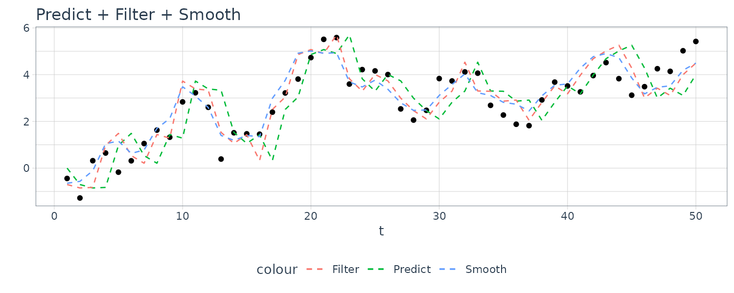
\[\begin{aligned} \textbf{x}_{t-1}^{n} &= \textbf{x}_{t-1}^{t-1} + \textbf{J}_{t-1}(\textbf{x}_{t}^{n} - \textbf{x}_{t}^{t-1})\\ \textbf{P}_{t-1}^{n} &= \textbf{P}_{t-1}^{t-1} + \textbf{J}_{t-1}(\textbf{P}_{t}^{n} - \textbf{P}_{t}^{t-1})\textbf{J}_{t-1}^{T} \end{aligned}\] \[\begin{aligned} \textbf{J}_{t-1} &= \textbf{P}_{t-1}^{t-1}\textbf{G}_{t}^{T}[\textbf{P}_{t}^{t-1}]^{-1} \end{aligned}\]

Example: Prediction, Filtering and Smoothing for the Local Level Model

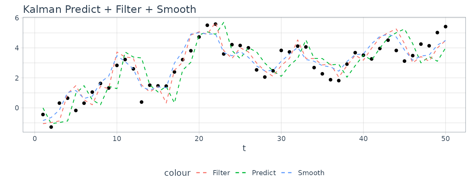
Suppose that we observe a univariate series \(y_{t}\) that consists of a trend component, \(\mu_{t}\), and a noise component, \(v_{t}\), where:

\[\begin{aligned} y_{t} &= \mu_{t} + v_{t} \end{aligned}\] \[\begin{aligned} v_{t} &\sim N(0, \sigma_{v}^{2}) \end{aligned}\]

We assume the trend is a random walk:

\[\begin{aligned} \mu_{t} &= \mu_{t-1}+ w_{t} \end{aligned}\] \[\begin{aligned} w_{t} &\sim N(0, \sigma_{w}^{2}) \end{aligned}\]

And \(w_{t}, v_{t}\) are independent of each other.

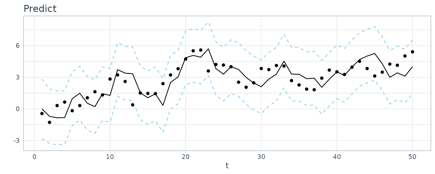
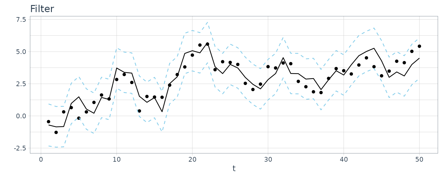
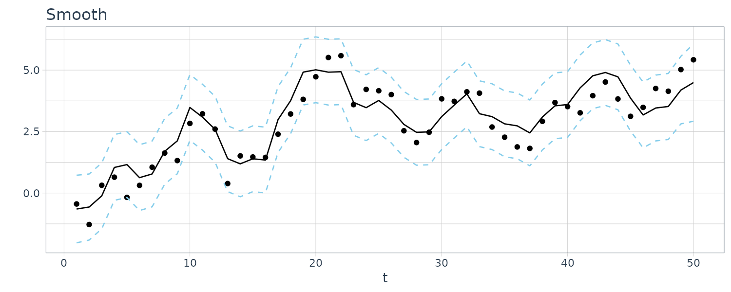
For this example, we simulated n = 50 observations from the above local level trend model. We generated a random walk:

\[\begin{aligned} \mu_{t} &= \mu_{t-1} + w_{t} \end{aligned}\] \[\begin{aligned} w_{t} &\sim N(0, 1)\\ \mu_{0} &\sim N(0, 1) \end{aligned}\]

We then supposed that we observe a univariate series \(y_{t}\) consisting of the trend component, \(\mu_{t}\), and a noise component \(v_{t}\) where:

\[\begin{aligned} y_{t} &= \mu_{t} + v_{t} \end{aligned}\] \[\begin{aligned} v_{t} &\sim N(0, 1) \end{aligned}\]

We then ran the Kalman filter and smoother:

\[\begin{aligned} \boldsymbol{\mu}_{t}^{t-1} &= \textbf{G}_{t} \boldsymbol{\mu}_{t-1}^{t-1}\\ \textbf{P}_{t}^{t-1} &= \textbf{G}_{t} \textbf{P}_{t-1}^{t-1}\textbf{G}_{t}^{T} + \textbf{W}_{t} \end{aligned}\] \[\begin{aligned} \boldsymbol{\mu}_{t}^{t} &= \boldsymbol{\mu}_{t}^{t-1} + \textbf{K}_{t}(y_{t} - \textbf{F}_{t}\boldsymbol{\mu}_{t}^{t-1})\\ \textbf{P}_{t}^{t} &= [\textbf{I} - \textbf{K}_{t}\textbf{F}_{t}]\textbf{P}_{t}^{t-1}\\ \textbf{K}_{t} &= \textbf{P}_{t}^{t-1}\textbf{F}_{t}^{T}[\textbf{F}_{t}\textbf{P}_{t}^{t-1}\textbf{F}_{t}^{T} + \textbf{V}_{t}]^{-1} \end{aligned}\] \[\begin{aligned} \boldsymbol{\mu}_{t-1}^{n} &= \boldsymbol{\mu}_{t-1}^{t-1} + \textbf{J}_{t-1}(x_{t}^{n} - \boldsymbol{\mu}_{t}^{t-1})\\ \textbf{P}_{t-1}^{n} &= \textbf{P}_{t-1}^{t-1} + \textbf{J}_{t-1}(\textbf{P}_{t}^{n} - \textbf{P}_{t}^{t-1})\textbf{J}_{t-1}^{T} \end{aligned}\] \[\begin{aligned} \textbf{J}_{t-1} &= \textbf{P}_{t-1}^{t-1}\textbf{G}_{t}^{T}[\textbf{P}_{t}^{t-1}]^{-1} \end{aligned}\]

Note that one-step-ahead prediction is more uncertain than the corresponding filtered value, which, in turn, is more uncertain than the corresponding smoother value:

\[\begin{aligned} \textbf{P}_{t}^{t-1} \geq \textbf{P}_{t}^{t} \geq \textbf{P}_{t}^{n} \end{aligned}\]

However, in each case, the error variances stabilize quickly.

Doing this in R:

set.seed(1)
num <- 50
w <- rnorm(num + 1, 0, 1)
v <- rnorm(num, 0, 1)

mu <- cumsum(w)
y <- mu[-1] + v

ks <- Ksmooth(
  y,
  A = 1,
  mu0 = 0,
  Sigma0 = 1,
  Phi = 1,
  sQ = 1,
  sR = 1
)

dat <- tsibble(
  t = 1:num,
  mu = mu[-1],
  Xp = as.numeric(ks$Xp),
  Xf = as.numeric(ks$Xf),
  Xs = as.numeric(ks$Xs),
  Pp = as.numeric(ks$Pp),
  Pf = as.numeric(ks$Pf),
  Ps = as.numeric(ks$Ps),    
  index = t
)

Similarly, we can do this using the dlm package in R:

dat <- tsibble(
  y = y,
  mu = mu[-1],
  t = 1:num,
  index = t
)

mod <- dlmModPoly(order = 1)

build_dlm <- function(par) {
  mod$W[1, 1] <- exp(par[1])
  mod$V[1, 1] <- exp(par[2])

  return(mod)
}

fit_dlm <- dlmMLE(
  y = dat$y,
  parm = c(0, 0),
  build = build_dlm,
  hessian = TRUE
)
fit_dlm

dlmFiltered_obj <- dlmFilter(
  y = dat$y,
  mod = mod
)
dlmFiltered_obj

dlmSmoothed_obj <- dlmSmooth(
  y = dat$y,
  mod = mod
)
dlmSmoothed_obj

dat <- dat |>
  mutate(
    a = dlmFiltered_obj$a,
    a_sdev = c(
      NA,
      sqrt(
        dropFirst(
          as.numeric(
            dlmSvd2var(
              dlmFiltered_obj$U.R,
              dlmFiltered_obj$D.R
            )
          )
        )
      )
    ),
    m = dropFirst(dlmFiltered_obj$m),     
    m_sdev = sqrt(
      dropFirst(
        as.numeric(
          dlmSvd2var(
            dlmFiltered_obj$U.C,
            dlmFiltered_obj$D.C
          )
        )
      )
    ),
    s = dropFirst(dlmSmoothed_obj$s),
    s_sdev = sqrt(
      dropFirst(
        as.numeric(
          dlmSvd2var(
            dlmSmoothed_obj$U.S,
            dlmSmoothed_obj$D.S
          )
        )
      )
    )
  )

Maximum Likelihood Estimation

Estimation of the parameters that specify the state space model is quite involved:

\[\begin{aligned} \textbf{x}_{t} &= \textbf{G}_{t}\textbf{x}_{t-1} + \Psi\textbf{u}_{t} + \boldsymbol{w}_{t}\\ \textbf{y}_{t} &= \textbf{F}_{t}\textbf{x}_{t-1} + \boldsymbol{\Gamma}_{t}\textbf{u}_{t} + \boldsymbol{v}_{t} \end{aligned}\]

We use \(\boldsymbol{\Theta}\) to represent the vector of unknown parameters, the initial mean and covariance \(\textbf{m}_{0}\) and \(\textbf{C}_{0}\) , the transition matrix \(\textbf{G}_{t}\), and the state and observation covariance matrices \(\textbf{W}_{t}\) and \(\textbf{V}_{t}\) and the input coefficient matrices, \(\Psi\) and \(\boldsymbol{\Gamma}_{t}\).

We use maximum likelihood under the assumption that the initial state is normal, \(\textbf{x}_{0} \sim N_{p}(\boldsymbol{\mu}_{0}, \textbf{C}_{0})\), and the errors are normal, \(\textbf{w}_{t} \sim N_{p}(\textbf{0}, \textbf{W}_{t})\) and \(\textbf{v}_{t} \sim N_{q}(\textbf{0}, \textbf{V}_{t})\).

We continue to assume, for simplicity, \(\textbf{w}_{t}, \textbf{v}_{t}\) are uncorrelated.

The likelihood is computed using the innovations \(e_{1}, e_{2}, \cdots, e_{n}\) (for linear models, maximizing the likelihood is the same as minimizing the sum of squares):

\[\begin{aligned} \textbf{e}_{t} &= \textbf{y}_{t} - \textbf{F}_{t}\textbf{x}_{t}^{t-1} - \boldsymbol{\Gamma}_{t} \textbf{u}_{t} \end{aligned}\]

The innovations form of the likelihood of the data \(\textbf{y}_{1:n}\), proceeds by noting the innovations are independent Gaussian random vectors with zero means and, covariance matrices:

\[\begin{aligned} \textbf{C}_{t} &\equiv \textrm{var}(\textbf{e}_{t})\\ &= \textrm{var}(\textbf{F}_{t}\textbf{x}_{t} + \textbf{v}_{t} - \textbf{F}_{t}\textbf{x}_{t}^{t-1}))\\ &= \textrm{var}(\textbf{F}_{t}(\textbf{x}_{t} - \textbf{x}_{t}^{t-1}) + \textbf{v}_{t})\\ &= \textbf{F}_{t}\textbf{P}_{t}^{t-1}\textbf{F}_{t}^{T} + \textbf{V}_{t} \end{aligned}\]

Hence, ignoring a constant, we may write the likelihood, \(L_{Y}(\boldsymbol{\Theta})\), as:

\[\begin{aligned} -\ln(L_{Y}(\boldsymbol{\Theta})) &= \frac{1}{2}\sum_{t=1}^{n}\ln|\textbf{C}_{t}(\boldsymbol{\Theta})| + \frac{1}{2}\sum_{t=1}^{n}\textbf{e}_{t}(\boldsymbol{\Theta})^{T}\textbf{C}_{t}(\boldsymbol{\Theta})^{-1}\textbf{e}_{t}(\boldsymbol{\Theta}) \end{aligned}\]

Where we have emphasized the dependence of the innovations on the parameters \(\boldsymbol{\Theta}\). The likelihood is a highly nonlinear and complicated function of the unknown parameters.

The usual procedure is to fix \(\textbf{x}_{0}\) and then develop a set of recursions for the log likelihood function and its first two derivatives. Then, a Newton–Raphson algorithm can be used successively to update the parameter values until the negative of the log likelihood is minimized.

The steps involved in performing a Newton–Raphson estimation procedure are as follows:

• Select initial values for the parameters, say, \(\boldsymbol{\Theta}(0)\).
• Run the Kalman filter, using the initial parameter values, \(\boldsymbol{\Theta}(0)\), to obtain a set of innovations and error covariances, say, \(\{e_{t}^{(0)}; t = 1, \cdots, n\}\) and \(\{\textbf{C}_{t}^{(0)}; t = 1, \cdots, n\}\).
• Run one iteration of a Newton–Raphson procedure with \(−\ln L_{Y}(\boldsymbol{\Theta})\) as the criterion function, to obtain a new set of estimates, say \(\boldsymbol{\Theta}(1)\).
• At iteration \(j\), (\(j = 1, 2, \cdots\)), repeat step 2 using \(\boldsymbol{\Theta}^{(j)}\) in place of \(\boldsymbol{\Theta}^{(j−1)}\) to obtain a new set of innovation values \(\{e_{t}; t = 1, \cdots, n\}\) and \(\{\textbf{C}_{t}; t = 1, \cdots, n\}\). Then repeat step 3 to obtain a new estimate \(\boldsymbol{\Theta}^{(j+1)}\). Stop when the estimates or the likelihood stabilize.

Example 6.6 Newton–Raphson for AR(1) Process with Observational Noise

Consider a univariate state-space model where the observations are noisy:

\[\begin{aligned} y_{t} &= x_{t} + v_{t} \end{aligned}\]

And the signal/state is an AR(1) process:

\[\begin{aligned} x_{t} &= \phi x_{t-1} + w_{t} \end{aligned}\] \[\begin{aligned} v_{t} &\sim N(0, \sigma_{v}^{2})\\ w_{t} &\sim N(0, \sigma_{w}^{2}) \end{aligned}\] \[\begin{aligned} x_{0} &\sim N\Big(0, \frac{\sigma_{w}^{2}}{1 - \phi^{2}}\Big) \end{aligned}\]

Recall if \(x_{t}\) is a stationary AR(1) process, the autocovariance function is:

\[\begin{aligned} \gamma_{x}(h) &= \frac{\sigma_{w}^{2}}{1 - \phi^{2}}\phi^{h} \end{aligned}\]

And the variance of \(y_{t}\):

\[\begin{aligned} \gamma_{y}(0) &= \textrm{var}(y_{t})\\ &= \textrm{var}(x_{t} + v_{})\\ &= \frac{\sigma_{w}^{2}}{1 - \phi^{2}} + \sigma_{v}^{2} \end{aligned}\]

And when \(h\geq 1\):

\[\begin{aligned} \gamma_{y}(h) &= \textrm{cov}(y_{t}, y_{t-h})\\ &= \textrm{cov}(x_{t} + v_{t}, x_{t-h} + v_{t-h})\\ &= \gamma_{x}(h) \end{aligned}\]

And the ACF:

\[\begin{aligned} \rho_{y}(h) &= \frac{\gamma_{y}(h)}{\gamma_{y}(0)}\\ &= \frac{\frac{\sigma_{w}^{2}}{1 - \phi^{2}}\phi^{h}}{\frac{\sigma_{w}^{2}}{1-\phi^{2}} + \sigma_{v}^{2}}\\ &= \frac{\phi^{h}}{1 + \frac{\sigma_{v}^{2}}{\sigma_{w}^{2}}(1 - \phi^{2})} \end{aligned}\]

The actual values of the parameters are (which we are going to estimate):

\[\begin{aligned} \phi &= 0.8 \end{aligned}\] \[\begin{aligned} \sigma_{w}^{2} &= 1\\ \sigma_{v}^{2} &= 1 \end{aligned}\]

In the simple case of an AR(1) with observational noise, we set the initial estimation:

\[\begin{aligned} \phi^{(0)} &= \frac{\hat{\rho}_{y}(2)}{\hat{\rho}_{y}(1)} \end{aligned}\] \[\begin{aligned} \sigma_{w}^{2^{(0)}} &= \frac{(1 - \phi^{(0)^{2}})\hat{\gamma}_{y}(1)}{\phi^{(0)}}\\ \sigma_{v}^{2^{(0)}} &= \hat{\gamma}_{y}(0) - \frac{\sigma_{w}^{2^{(0)}}}{1 - \phi^{(0)^{2}}} \end{aligned}\]

For \(\phi^{(0)}\), we know that:

\[\begin{aligned} \frac{\rho_{y}(2)}{\rho_{y}(1)} &= \frac{\phi^{2}}{\phi}\\ &= \phi \end{aligned}\]

For \(\sigma_{w}^{2^{(0)}}\), we know that:

\[\begin{aligned} \gamma_{x}(1) &= \gamma_{y}(1)\\ &= \frac{\sigma_{w}^{2}}{1 - \phi^{2}}\phi\\ \sigma_{w}^{2} &= \frac{1 - \phi^{2}}{\phi}\gamma_{y}(1) \end{aligned}\]

And for \(\sigma_{v}^{2^{(0)}}\) we know that:

\[\begin{aligned} \gamma_{y}(0) &= \frac{\sigma_{w}^{2}}{1 - \phi^{2}} + \sigma_{v}^{2}\\ \sigma_{v}^{2} &= \gamma_{y}(0) - \frac{\sigma_{w}^{2}}{1 - \phi^{2}} \end{aligned}\]

Newton–Raphson estimation was accomplished using the R program optim. In that program, we must provide an evaluation of the function to be minimized, namely, \(−\ln L_{Y}(\boldsymbol{\Theta})\). In this case, the function call combines steps 2 and 3, using the current values of the parameters, \(\boldsymbol{\Theta}(j−1)\), to obtain first the filtered values, then the innovation values, and then calculating the criterion function, \(−\ln L_{Y}(\boldsymbol{\Theta}(j−1))\), to be minimized.

We can also provide analytic forms of the gradient or score vector, \(−\frac{\partial \ln L_{Y}(\boldsymbol{\Theta})}{\partial \boldsymbol{\Theta}}\), and the Hessian matrix, \(−\frac{\partial 2 \ln L_{Y}(\boldsymbol{\Theta})}{\partial\boldsymbol{\Theta} \partial\boldsymbol{\Theta}^{T}}\), in the optimization routine, or allow the program to calculate these values numerically.

In this example, we let the program proceed numerically and we note the need to be cautious when calculating gradients numerically. It it suggested that it is better to use numerical methods for the derivatives, at least for the Hessian, along with the Broyden–Fletcher–Goldfarb–Shanno (BFGS) method.

Simulating the data in R using actual values:

set.seed(999)
num <- 100
x <- arima.sim(
  n = num + 1,
  list(ar = .8),
  sd = 1
)

dat <- tsibble(
  t = 1:num,
  x = x[-1],
  y = x[-1] + rnorm(num, 0, 1),   
  index = t
)

dat <- dat |>
  mutate(
    y1 = lag(y),
    y2 = lag(y, 2)
  )

We are computing lags to compute the ACF values. Using optim and returning the Hessian matrix in order to calculate SE:

# Initial Estimates
u <- dat |>
  slice(3:n()) |>
  as_tibble() |>
  select(y, y1, y2)

varu <- var(u)
coru <- cor(u)

acfs <- dat |>
  feasts::ACF(y) |>
  pull(acf)

phi <- coru[1, 3] / coru[1, 2]
q <- (1 - phi^2) * varu[1, 2] / phi
r <- varu[1, 1] - q / (1 - phi^2)
init.par <- c(phi, sqrt(q), sqrt(r))

> init.par
[1] 0.9087024 0.5107053 1.0291205

# Function to evaluate the likelihood
Linn <- function(para) {
  phi <- para[1]
  sigw <- para[2]
  sigv <- para[3]
  Sigma0 <- (sigw^2) / (1 - phi^2)
  Sigma0[Sigma0 < 0] <- 0

  kf <- Kfilter(dat$y, 1, mu0 = 0, Sigma0, phi, sigw, sigv)     

  return(kf$like)
}

est <- optim(
  init.par,
  Linn,
  gr = NULL,
  method = "BFGS",
  hessian = TRUE,
  control = list(trace = 1, REPORT = 1)
)

> est
$par
[1] 0.8137623 0.8507863 0.8743968

$value
[1] 79.01445

$counts
function gradient 
      23        7 

$convergence
[1] 0

$message
NULL

$hessian
          [,1]     [,2]     [,3]
[1,] 253.36290 67.39775 -9.64101
[2,]  67.39775 78.99067 48.61052
[3,]  -9.64101 48.61052 92.20472

SE <- sqrt(diag(solve(est$hessian)))

> cbind(
  estimate = c(
    phi = est$par[1],
    sigw = est$par[2],
    sigv = est$par[3]),
  SE
)
      estimate         SE
phi  0.8137623 0.08060636
sigw 0.8507863 0.17528895
sigv 0.8743968 0.14293192

We can see the values are similar to the actual values.

We can do the same using dlm package:

library(dlm)

mod <- dlmModPoly(order = 1)

build_dlm <- function(par) {
  mod$GG[1, 1] <- par[1]
  mod$W[1, 1] <- par[2]
  mod$V[1, 1] <- par[3]

  return(mod)
}

phi <- init.par[1]
sigw <- init.par[2]
sigv <- init.par[3]
Sigma0 <- (sigw^2) / (1 - phi^2)
mod$C0 <- Sigma0

fit_dlm <- dlmMLE(
  y = dat$y,
  parm = init.par,
  build = build_dlm,
  method = "BFGS",
  hessian = TRUE
)

> fit_dlm
$par
[1] 0.8158753 0.7105982 0.7755896

$value
[1] 79.04665

$counts
function gradient 
      20        8 

$convergence
[1] 0

$message
NULL

$hessian
           [,1]     [,2]      [,3]    
[1,] 246.614632 38.91043 -6.502895
[2,]  38.910425 27.63736 16.003478
[3,]  -6.502895 16.00348 29.832270

Example: Newton–Raphson for the Global Temperature Deviations

Recall the earlier example:

The above figure shows two different estimators for the global temperature series from 1880 to 2015. One is globtemp which contains the global mean land-ocean temperature index data. The second series, globtempl, are the surface air temperature index data using only meteorological station data.

Conceptually, both series should be measuring the same underlying climatic signal, and we may consider the problem of extracting this underlying signal.

We suppose both series are observing the same signal with different noises:

\[\begin{aligned} y_{t1} &= x_{t} + v_{t1}\\ y_{t2} &= x_{t} + v_{t2} \end{aligned}\] \[\begin{aligned} \begin{bmatrix} y_{t1}\\ y_{t2} \end{bmatrix} &= \begin{bmatrix} 1\\ 1 \end{bmatrix}x_{t} + \begin{bmatrix} v_{t1}\\ v_{t2} \end{bmatrix} \end{aligned}\]

And \(v_{t}\) having the covariance matrix \(\textbf{V}_{t}\):

\[\begin{aligned} \textbf{V}_{t} &= \begin{bmatrix} V_{11} & V_{12}\\ V_{21} & V_{22} \end{bmatrix} \end{aligned}\]

We further assume and model \(x_{t}\) as a random walk with drift

\[\begin{aligned} x_{t} &= \delta + x_{t-1} + w_{t} \end{aligned}\]

And variance \(\textbf{W}_{t}\):

\[\begin{aligned} \textbf{W}_{t} = \text{var}(w_{t}) \end{aligned}\]

Hence, there are five parameters to estimate, \(\delta\), the drift, and the variance components, \(V_{11}, V_{12}, V_{21}, V_{22}\), noting that \(V_{21} = r_{12}\).

To summarize, the following are the DLM parameters:

\[\begin{aligned} \textbf{G}_{t} &= \begin{bmatrix} 1 \end{bmatrix}\\ \textbf{W}_{t} &= \begin{bmatrix} \sigma_{w_{t}} \end{bmatrix}\\ \textbf{y}_{t} &= \begin{bmatrix} y_{t1}\\ y_{t2} \end{bmatrix}\\ \textbf{F}_{t} &= \begin{bmatrix} 1\\ 1 \end{bmatrix}\\ \textbf{V}_{t} &= \begin{bmatrix} V_{11} & V_{12}\\ V_{21} & V_{22} \end{bmatrix}\\ \boldsymbol{\Psi}_{t} &= \begin{bmatrix} 1 \end{bmatrix}\\ \boldsymbol{\Gamma}_{t} &= \begin{bmatrix} 1 \end{bmatrix} \end{aligned}\]

We hold the the initial state parameters fixed in this example at:

\[\begin{aligned} \boldsymbol{\mu}_{0} &= -0.35\\ \textbf{C}_{0} &= 1 \end{aligned}\]

Which is large relative to the data.

Let’s code this in R. Note that in the likelihood function, we specify Cholesky-type decomposition for Q and R. They can be reconstructed by:

t(cQ) %*% cQ
t(cR) %*% cR  

The code:

y <- cbind(globtemp, globtempl)
num <- nrow(y)

input <- rep(1, num)
A <- array(rep(1, 2), dim = c(2, 1, num))

mu0 <- -.35
Sigma0 <- 1
Phi <- 1

# Function to Calculate Likelihood
Linn <- function(para) {
  cQ <- para[1]
  cR1 <- para[2]
  cR2 <- para[3]
  cR12 <- para[4]
  # put the matrix together
  cR <- matrix(c(cR1, 0, cR12, cR2), 2)
  drift <- para[5]

  kf <- Kfilter(
    y,
    A,
    mu0,
    Sigma0,
    Phi,
    Ups = drift,
    sQ = t(cQ),
    sR = t(cR),
    input = input
  )

  return(kf$like)
}

# Estimation
# initial values of parameters
init.par <- c(.1, .1, .1, 0, .05)
est <- optim(
  init.par,
  Linn,
  NULL,
  method = "BFGS",
  hessian = TRUE,
  control = list(trace = 1, REPORT = 1)
)
est

SE <- sqrt(diag(solve(est$hessian)))
# Display estimates
u <- cbind(estimate = est$par, SE)
rownames(u) <- c("sigw", "cR11", "cR22", "cR12", "drift")    

> u
        estimate          SE
sigw  0.05501124 0.011358852
cR11  0.07418174 0.009856923
cR22  0.12694400 0.015481675
cR12  0.12925308 0.038230357
drift 0.00649545 0.004787053

# Smooth (first set parameters to their final estimates)
cQ <- est$par[1]
cR1 <- est$par[2]
cR2 <- est$par[3]
cR12 <- est$par[4]
cR <- matrix(c(cR1, 0, cR12, cR2), 2)
R <- t(cR) %*% cR

> R
            [,1]        [,2]
[1,] 0.005502931 0.009588218
[2,] 0.009588218 0.032821136

We proceed to plot the smoothed estimate of the signal \(\hat{x}_{t}^{n}\):

ks <- Ksmooth(
  y,
  A,
  mu0,
  Sigma0,
  Phi,
  t(cQ),
  t(cR),
  Ups = drift,
  input = input
)

dat <- tsibble(
  t = seq(
    as.Date("1880-01-01"),
    as.Date("2015-01-01"),
    by = "1 year") |>
    year(),
  xsm = as.vector(ks$Xs),
  rmse = sqrt(as.vector(ks$Ps)),    
  globtemp = globtemp,
  globtempl = globtempl,
  index = t
)

Note only values after 1900 is shown:

Expectation-Maximization (EM) Algorithm

In addition to Newton–Raphson, Shumway and Stoffer presented a conceptually simpler estimation procedure based on the Baum-Welch algorithm known as the EM (expectation-maximization) algorithm.

The basic idea is that if we could observe the states, \(x_{0:n} = \{x_{0}, x_{1}, \cdots, x_{n}\}\), in addition to the observations \(y_{1:n} = \{y1, \cdots, y_{n}\}\), then we would consider \(\{x_{0:n}, y_{1:n}\}\) as the complete data, with joint density:

\[\begin{aligned} \textbf{P}_{\boldsymbol{\Theta}}(x_{0:n}, y_{1:n}) &= \textbf{P}_{\boldsymbol{\mu}_{0}, \textbf{C}_{0}}(x_{0})\prod_{t=1}^{n}p_{\textbf{G}_{t}, \textbf{W}_{t}}(x_{t}|x_{t-1})\prod_{t=1}^{n}p_{\textbf{V}_{t}}(y_{t}|x_{}) \end{aligned}\]

Under the Gaussian assumption and ignoring constants, the complete data likelihood can be written as:

\[\begin{aligned} -2\ln L_{X, Y}(\boldsymbol{\Theta}) =\ &\ln|\textbf{C}_{0}| + (x_{t} - \boldsymbol{\mu}_{0})^{T}\textbf{C}_{0}^{-1}(x_{t} - \boldsymbol{\mu}_{0})\\ \ &+ n\ln|\textbf{W}_{t}| + \sum_{t=1}^{n}(x_{t} - \textbf{G}_{t} x_{t-1})^{T}\textbf{W}_{t}^{-1}(x_{t} - \textbf{G}_{t} x_{t-1})\\ \ &+ n\ln|\textbf{V}_{t}| + \sum_{t=1}^{n}(y_{t} - \textbf{F}_{t} x_{t})^{T}\textbf{V}_{t}^{-1}(y_{t} - \textbf{F}_{t} x_{t}) \end{aligned}\]

If we did have the complete data, we could then use the results from multivariate normal theory to easily obtain the MLEs of \(\boldsymbol{\Theta}\). Although we do not have the complete data, the EM algorithm gives us an iterative method for finding the MLEs of \(\boldsymbol{\Theta}\) based on the incomplete data, \(y_{1:n}\), by successively maximizing the conditional expectation of the complete data likelihood.

The simple explanation for the EM algorithm is that it is simply alternating between the Kalman filtering and smoothing recursions and the multivariate normal maximum likelihood estimators.

EM Algorithm for for AR(1) Process with Observational Noise

Recall the state-space model example where the observations are noisy:

\[\begin{aligned} y_{t} &= x_{t} + v_{t} \end{aligned}\]

And the signal/state is an AR(1) process:

\[\begin{aligned} x_{t} &= \phi x_{t-1} + w_{t} \end{aligned}\]

Evaluation of the standard errors used a call to fdHess in the nlme R package to evaluate the Hessian at the final estimates.

em <- EM(
  dat$y,
  A = 1,
  mu0 = 0,
  Sigma0 = 2.8,
  Phi = phi,
  Q = q,
  R = r,
  max.iter = 75,
  tol = .00001
)

> em
$Phi
[1] 0.8097511

$Q
[1] 0.7280685

$R
          [,1]
[1,] 0.7457129

$mu0
          [,1]
[1,] -1.964872

$Sigma0
           [,1]
[1,] 0.02227538

$like
 ...

$niter
[1] 74

$cvg
[1] 9.989903e-06

# Standard Errors (this uses nlme)
phi <- em$Phi
sq <- sqrt(em$Q)
sr <- sqrt(em$R)
mu0 <- em$mu0
Sigma0 <- em$Sigma0
para <- c(phi, sq, sr)

Linn <- function(para) {
  kf <- Kfilter(
    dat$y,
    1,
    mu0,
    Sigma0,
    para[1],
    para[2],
    para[3]
  )

  return(kf$like)
}

emhess = fdHess(
  para,
  function(para) {
    Linn(para)
  }
)

> emhess
$mean
[1] 78.02873

$gradient
[1]  0.02944336 -0.05996481  0.04564833   

$Hessian
          [,1]     [,2]      [,3]
[1,] 247.71935 63.14721 -11.17437
[2,]  63.14721 80.94489  48.10926
[3,] -11.17437 48.10926  94.14988

SE <- sqrt(diag(solve(emhess$Hessian)))

# Display Summary of Estimation
estimate <- c(para, em$mu0, em$Sigma0)
SE <- c(SE, NA, NA)
u <- cbind(estimate, SE)
rownames(u) <- c("phi", "sigw", "sigv", "mu0", "Sigma0")    

> u
          estimate         SE
phi     0.80975110 0.07850196
sigw    0.85326930 0.16413552
sigv    0.86354667 0.13658590
mu0    -1.96487182         NA
Sigma0  0.02227538         NA

Missing Data Modifications

An attractive feature available within the state space framework is its ability to treat time series that have been observed irregularly over time. For example, using the state-space representation to fit ARMA models to series with missing observations, and using the model for estimation and forecasting of ARFIMA series with missing observations.

Suppose, at a given time t, we define the partition of the q x 1 observation vector into two parts, \(y_{t}^{(1)}\), the \(q_{1t} \times 1\) component of observed values, and \(y_{t}^{2}\), the \(q_{2t} \times 1\) component of unobserved values, where \(q_{1t} + q_{2t} = q\). Then, write the partitioned observation equation as:

\[\begin{aligned} \begin{bmatrix} \textbf{y}_{t}^{(1)}\\ \textbf{y}_{t}^{(2)} \end{bmatrix} &= \begin{bmatrix} \textbf{F}_{t}^{(1)}\\ \textbf{F}_{t}^{(2)} \end{bmatrix}\textbf{x}_{t} + \begin{bmatrix} \textbf{v}_{t}^{(1)}\\ \textbf{v}_{t}^{(2)} \end{bmatrix} \end{aligned}\]

And covariance matrix of the measurement errors between the observed and unobserved parts:

\[\begin{aligned} \begin{bmatrix} V_{11t} & V_{12t}\\ V_{21t} & V_{22t} \end{bmatrix} \end{aligned}\]

In the missing data case where \(y^{t}^{(2)}\) is not observed, we may modify the observation equation in the DLM, so that the model is:

\[\begin{aligned} \textbf{x}_{t} &= \textbf{G}_{t}\textbf{x}_{t-1} + \textbf{w}_{t}\\ \textbf{y}_{t}^{(1)} &= \textbf{G}_{t}^{(1)}\textbf{x}_{t} + \textbf{v}_{t}^{(1)} \end{aligned}\]

Rather than deal with varying observational dimensions, it is computationally easier to modify the model by zeroing out certain components and retaining a q-dimensional observation equation throughout:

\[\begin{aligned} \textbf{y}_{t} &= \begin{bmatrix} \textbf{y}_{t}\\ \textbf{0} \end{bmatrix}\\ \textbf{G}_{t} &= \begin{bmatrix} \textbf{G}_{t}^{(1)}\\ \textbf{0} \end{bmatrix} \end{aligned}\]

Example: Longitudinal Biomedical Data

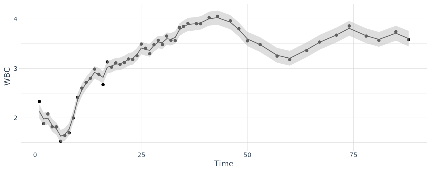
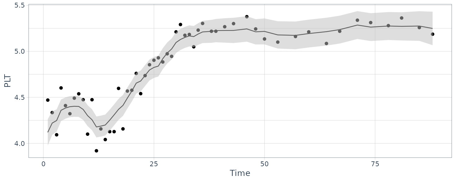
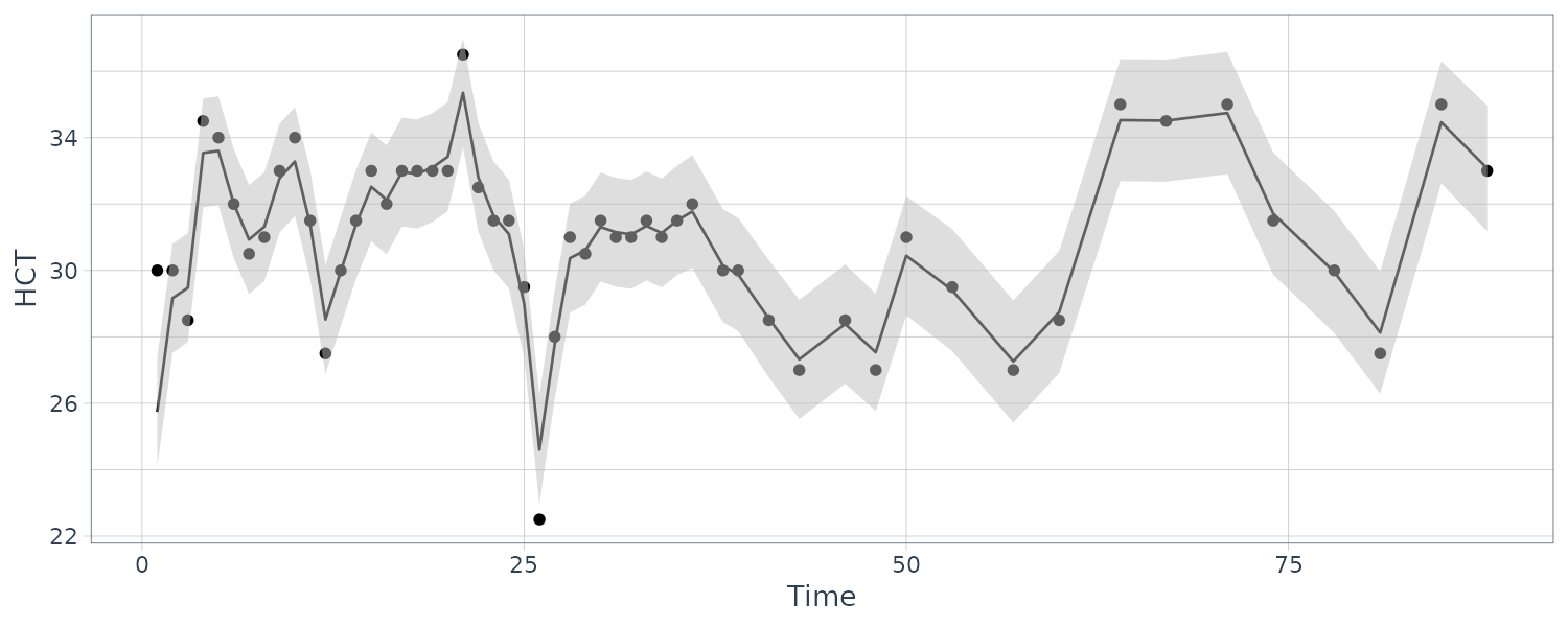
We consider the biomedical data, which have portions of the three dimensional vector missing after the 40th day.

The observation matrices \(A_{t}\) or \(F_{t}\) are either the identity or zero matrix because all the series are either observed or not observed:

y <- cbind(WBC, PLT, HCT)
num <- nrow(y)
# make array of obs matrices
A <- array(0, dim = c(3, 3, num))
for (k in 1:num) {
  # non-missing data
  if (y[k, 1] > 0) {
    A[, , k] <- diag(1, 3)
  }
}

# Initial values
mu0 <- matrix(0, 3, 1)
Sigma0 <- diag(
  c(.1, .1, 1),
  3
)
Phi <- diag(1, 3)
cQ <- diag(
  c(.1, .1, 1),
  3
)
cR <- diag(
  c(.1, .1, 1),
  3
)

# EM procedure
em <- EM(
  y,
  A,
  mu0,
  Sigma0,
  Phi,
  t(cQ) %*% cQ,
  t(cR) %*% cR,
  max.iter = 100,
  tol = .001
)

> em
$Phi
            [,1]        [,2]        [,3]
[1,]  0.98052698 -0.03494377 0.008287009
[2,]  0.05279121  0.93299479 0.005464917
[3,] -1.46571679  2.25780951 0.795200344

$Q
             [,1]         [,2]       [,3]
[1,]  0.013786772 -0.001724166 0.01882951
[2,] -0.001724166  0.003032109 0.03528162
[3,]  0.018829510  0.035281625 3.61897901

$R
            [,1]      [,2]      [,3]
[1,] 0.007124671 0.0000000 0.0000000
[2,] 0.000000000 0.0168669 0.0000000
[3,] 0.000000000 0.0000000 0.9724247

$mu0
          [,1]
[1,]  2.119269
[2,]  4.407390
[3,] 23.905038

$Sigma0
              [,1]          [,2]          [,3]
[1,]  4.553949e-04 -5.249215e-05  0.0005877626    
[2,] -5.249215e-05  3.136928e-04 -0.0001199788
[3,]  5.877626e-04 -1.199788e-04  0.1677365489

The coupling between the first and second series is relatively weak, whereas the third series HCT is strongly related to the first two; that is:

\[\begin{aligned} \hat{x}_{t3} &= -1.497 x_{t-1,1} + 2.258 x_{t-1,2} + 0.795 x_{t-1, 3} \end{aligned}\]

Hence, the HCT is negatively correlated with white blood count (WBC) and positively correlated with platelet count (PLT). Byproducts of the procedure are es timated trajectories for all three longitudinal series and their respective prediction intervals.

ks <- Ksmooth(
  y,
  A,
  mu0,
  Sigma0,
  Phi,
  t(chol(em$Q)),
  t(chol(em$R))
)

dat <- tsibble(
  WBC = y[, "WBC"],
  PLT = y[, "PLT"],
  HCT = y[, "HCT"],
  y1s = ks$Xs[1, , ],
  y2s = ks$Xs[2, , ],
  y3s = ks$Xs[3, , ],
  p1 = 2 * sqrt(ks$Ps[1, 1, ]),
  p2 = 2 * sqrt(ks$Ps[2, 2, ]),
  p3 = 2 * sqrt(ks$Ps[3, 3, ]),    
  t = 1:nrow(y),
  index = t
)

Structural Models: Signal Extraction and Forecasting

Structural models are component models in which each component may be thought of as explaining a specific type of behavior. The models are often some version of the classical time series decomposition of data into trend, seasonal, and irregular components. Consequently, each component has a direct interpretation as to the nature of the variation in the data.

Furthermore, the model fits into the state space framework quite easily. To illustrate these ideas, we consider an example that shows how to fit a sum of trend, seasonal, and irregular components to the quarterly earnings data that we have considered before.

Example: Johnson & Johnson Quarterly Earnings

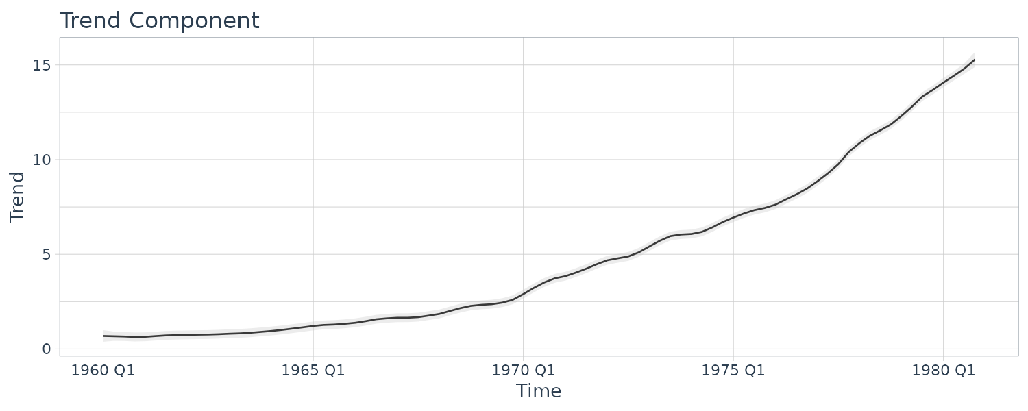
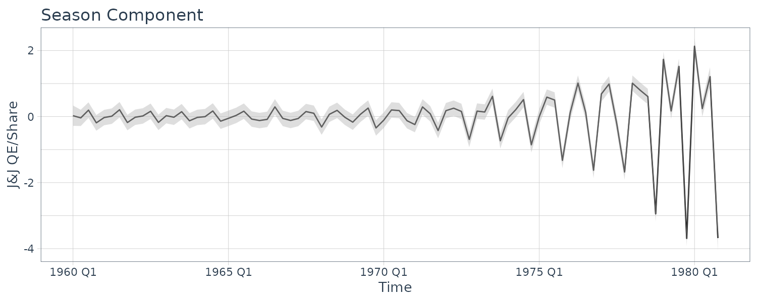
The Johnson & Johnson series is highly nonstationary, and there is both a trend signal that is gradually increasing over time and a seasonal component that cycles every four quarters or once per year. The seasonal component is getting larger over time as well. Transforming into logarithms or even taking the nth root does not seem to make the series trend stationary, however, such a transformation does help with stabilizing the variance over time.

Let the observed series be expressed as:

\[\begin{aligned} y_{T} &= T_{t} + S_{t} + v_{t} \end{aligned}\]

Suppose we allow the trend to increase exponentially:

\[\begin{aligned} T_{t} &= \phi T_{t-1} + w_{t1} \end{aligned}\] \[\begin{aligned} \phi &> 1 \end{aligned}\]

Let the seasonal component be modeled as:

\[\begin{aligned} S_{t} + S_{t-1} + S_{t-2} + S_{t-3} &= w_{t2} \end{aligned}\]

Which corresponds to assuming the component is expected to sum to zero over a complete period or four quarters.

To express this model in state-space form, let the following be the state vector:

\[\begin{aligned} x_{t} &= \begin{bmatrix} T_{t}\\ S_{t}\\ S_{t-1}\\ S_{t-2} \end{bmatrix} \end{aligned}\]

The observation equation can be written as:

\[\begin{aligned} y_{t} &= \begin{bmatrix} 1 & 1 & 0 & 0 \end{bmatrix} \begin{bmatrix} T_{t}\\ S_{t}\\ S_{t-1}\\ S_{t-2} \end{bmatrix} + v_{t} \end{aligned}\]

And the state equation:

\[\begin{aligned} \begin{bmatrix} T_{t}\\ S_{t}\\ S_{t-1}\\ S_{t-2} \end{bmatrix} &= \begin{bmatrix} \phi & 0 & 0 & 0\\ 0 & -1 & -1 & -1\\ 0 & 1 & 0 & 0\\ 0 & 0 & 1 & 0 \end{bmatrix} \begin{bmatrix} T_{t-1}\\ S_{t-1}\\ S_{t-2}\\ S_{t-3} \end{bmatrix} + \begin{bmatrix} w_{t1}\\ w_{t2}\\ 0\\ 0 \end{bmatrix} \end{aligned}\]

Where \(\textbf{V}_{t} = v_{11}\) and:

\[\begin{aligned} \textbf{W}_{t} = \begin{bmatrix} w_{11} & 0 & 0 & 0\\ 0 & w_{22} & 0 & 0\\ 0 & 0 & 0 & 0\\ 0 & 0 & 0 & 0 \end{bmatrix} \end{aligned}\]

The parameters to be estimated are \(v_{11}\), the noise variance in the measurement equations, \(w_{11}, w_{22}\), the model variances corresponding to the trend and seasonal components and \(\textbf{G}_{t}\), the transition parameter that models the growth rate.

Growth is about 3% per year, and so we began with \(\textbf{G}_{t} = 1.03\). The initial mean was fixed at:

\[\begin{aligned} \boldsymbol{\mu}_{0} &= \begin{bmatrix} 0.7\\ 0\\ 0\\ 0 \end{bmatrix} \end{aligned}\]

With uncertainty modeled by the diagonal covariance matrix:

\[\begin{aligned} \textbf{C}_{0} &= \begin{bmatrix} 0.04 & 0 & 0 & 0\\ 0 & 0.04 & 0 & 0\\ 0 & 0 & 0.04 & 0\\ 0 & 0 & 0 & 0.04 \end{bmatrix} \end{aligned}\]

Initial state covariance values were taken as \(w_{11} = .01\), \(w_{22} = .01\). The measurement error covariance was started at \(q_{11} = .25\).

num <- length(jj)
A <- cbind(1, 1, 0, 0)

# Function to Calculate Likelihood
Linn <- function(para) {
  Phi <- diag(0, 4)
  Phi[1, 1] <- para[1]
  Phi[2, ] <- c(0, -1, -1, -1)
  Phi[3, ] <- c(0, 1, 0, 0)
  Phi[4, ] <- c(0, 0, 1, 0)

  cQ1 <- para[2]
  cQ2 <- para[3]

  # sqrt q11 and q22
  cQ <- diag(0, 4)
  cQ[1, 1] <- cQ1
  cQ[2, 2] <- cQ2
  cR <- para[4]

  kf <- Kfilter(
    jj,
    A,
    mu0,
    Sigma0,
    Phi,
    t(cQ),
    t(cR)
  )

  return(kf$like)
}

# Initial Parameters
mu0 <- c(.7, 0, 0, 0)
Sigma0 <- diag(.04, 4)
init.par <- c(1.03, .1, .1, .5)

# Phi[1,1], the 2 cQs and cR
# Estimation and Results
est <- optim(
  init.par,
  Linn,
  NULL,
  method = "BFGS",
  hessian = TRUE,
  control = list(trace = 1, REPORT = 1)
)

SE <- sqrt(diag(solve(est$hessian)))
u <- cbind(estimate = est$par, SE)
rownames(u) <- c("Phi11", "sigw1", "sigw2", "sigv")    

> u
          estimate         SE
Phi11 1.0350847657 0.00253645
sigw1 0.1397255477 0.02155155
sigw2 0.2208782663 0.02376430
sigv  0.0004655672 0.24174702

After about 20 iterations of a Newton–Raphson, the transition parameter estimate was \(\hat{\textbf{G}_{t}} = 1.035\), corresponding to exponential growth with inflation at about 3.5% per year. The measurement uncertainty was small at \(\sqrt{\hat{v}_{11}} = 0.0005\), compared with the model uncertainties of \(\sqrt{\hat{w}_{11}} = 0.1397\) and \(\sqrt{\hat{w}_{22}} = 0.2209\).

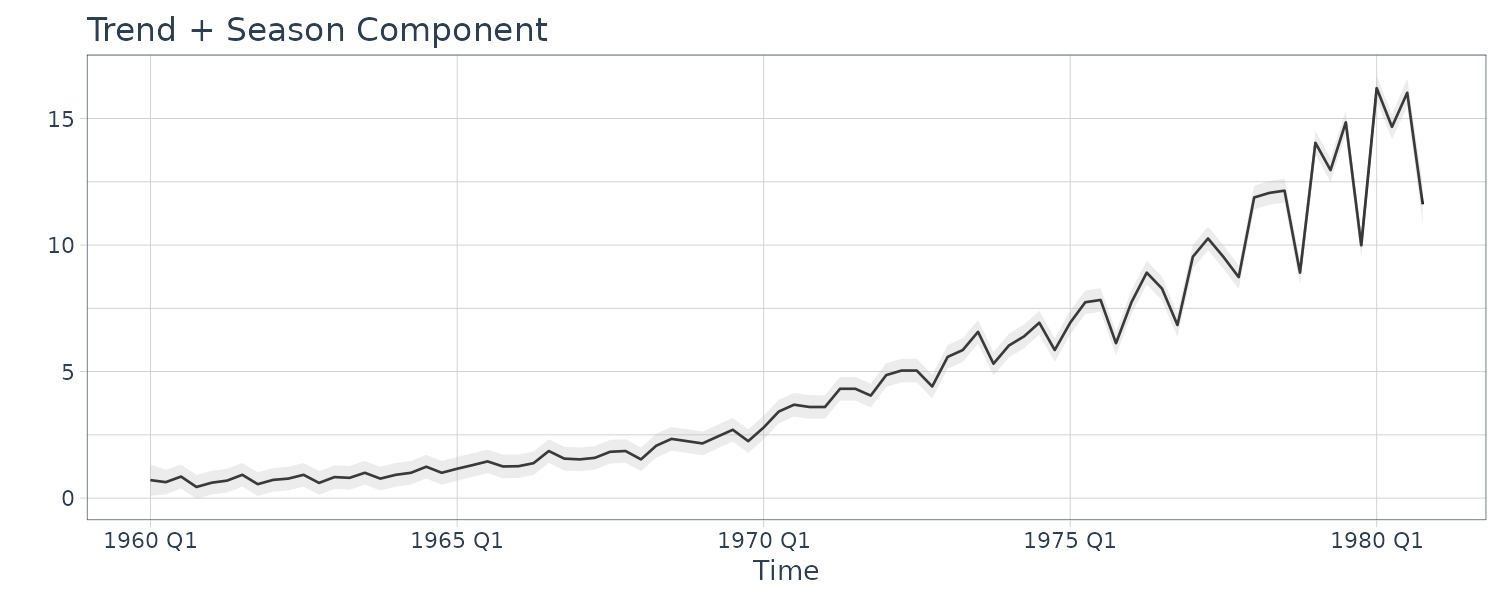
Plotting the smooth trend and season:

# Smooth
Phi <- diag(0, 4)
Phi[1, 1] <- est$par[1]
Phi[2, ] <- c(0, -1, -1, -1)
Phi[3, ] <- c(0, 1, 0, 0)
Phi[4, ] <- c(0, 0, 1, 0)
cQ1 <- est$par[2]
cQ2 <- est$par[3]
cQ <- diag(0, 4)
cQ[1, 1] <- cQ1
cQ[2, 2] <- cQ2
cR <- est$par[4]
ks <- Ksmooth(
  jj,
  A,
  mu0,
  Sigma0,
  Phi,
  t(cQ),
  t(cR)
)

# Plots
dat <- tsibble(
  t = seq(
    as.Date("1960-01-01"),
    as.Date("1980-12-01"),
    by = "1 quarter") |>
    yearquarter(),
  Tsm = as.vector(ks$Xs[1, , ]),    
  Ssm = as.vector(ks$Xs[2, , ]),
  p1 = 3 * sqrt(ks$Ps[1, 1, ]),
  p2 = 3 * sqrt(ks$Ps[2, 2, ]),
  jj = as.vector(jj),
  index = t
)

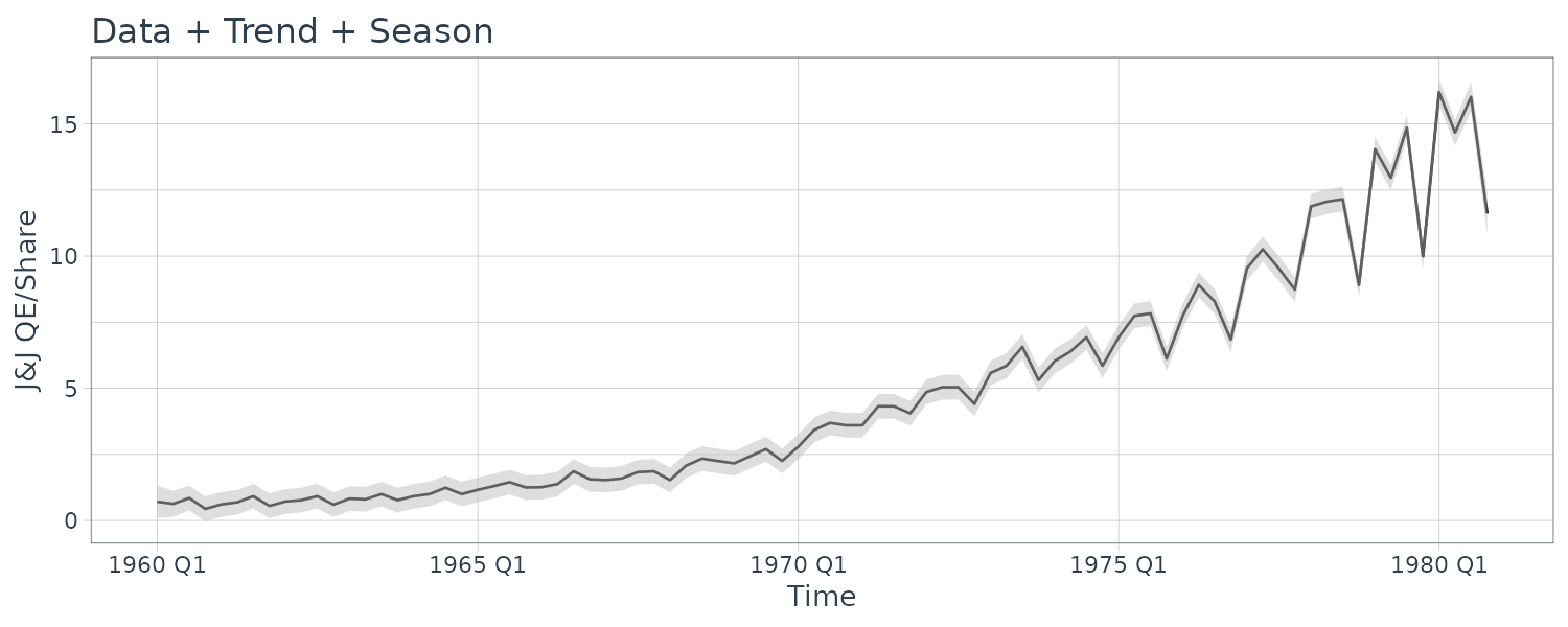
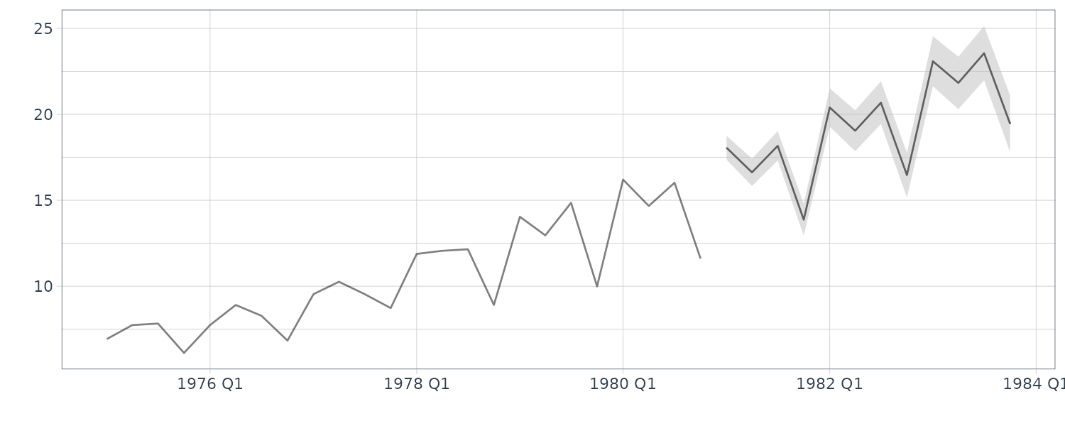
And the forecast for 12 quarters:

n.ahead <- 12
test_dat <- tsibble(
  t = seq(
    as.Date("1981-01-01"),
    as.Date("1983-12-01"),
    by = "1 quarter"
  ) |>
    yearquarter(),
  jj = rep(0, n.ahead),
  rmspe = rep(0, n.ahead),
  index = t
)

y <- ts(
  append(jj, rep(0, n.ahead)),
  start = 1960,
  freq = 4
)
rmspe <- rep(0, n.ahead)
x00 <- ks$Xf[, , num]
P00 <- ks$Pf[, , num]
Q <- t(cQ) %*% cQ
R <- t(cR) %*% (cR)

for (m in 1:n.ahead) {
  xp <- Phi %*% x00
  Pp <- Phi %*% P00 %*% t(Phi) + Q
  sig <- A %*% Pp %*% t(A) + R
  K <- Pp %*% t(A) %*% (1 / sig)
  x00 <- xp
  P00 <- Pp - K %*% A %*% Pp
  y[num + m] <- A %*% xp
  rmspe[m] <- sqrt(sig)
  test_dat$jj[m] <- A %*% xp
  test_dat$rmspe[m] <- sqrt(sig)
}

dat <- bind_rows(dat, test_dat)

dat |>
  filter(t >= yearquarter(as.Date("1975-01-01"))) |>    
  autoplot(jj) +
  geom_line(aes(y = y), data = test_dat) +
  xlab("Time") +
  ylab("J&J QE/Share") +
  ggtitle("Data + Trend + Season") +
  geom_ribbon(
    aes(
      ymax = jj + 3 * rmspe,
      ymin = jj - 3 * rmspe
    ),
    fill = "gray",
    alpha = 0.5,
    data = test_dat
  ) +
  theme_tq()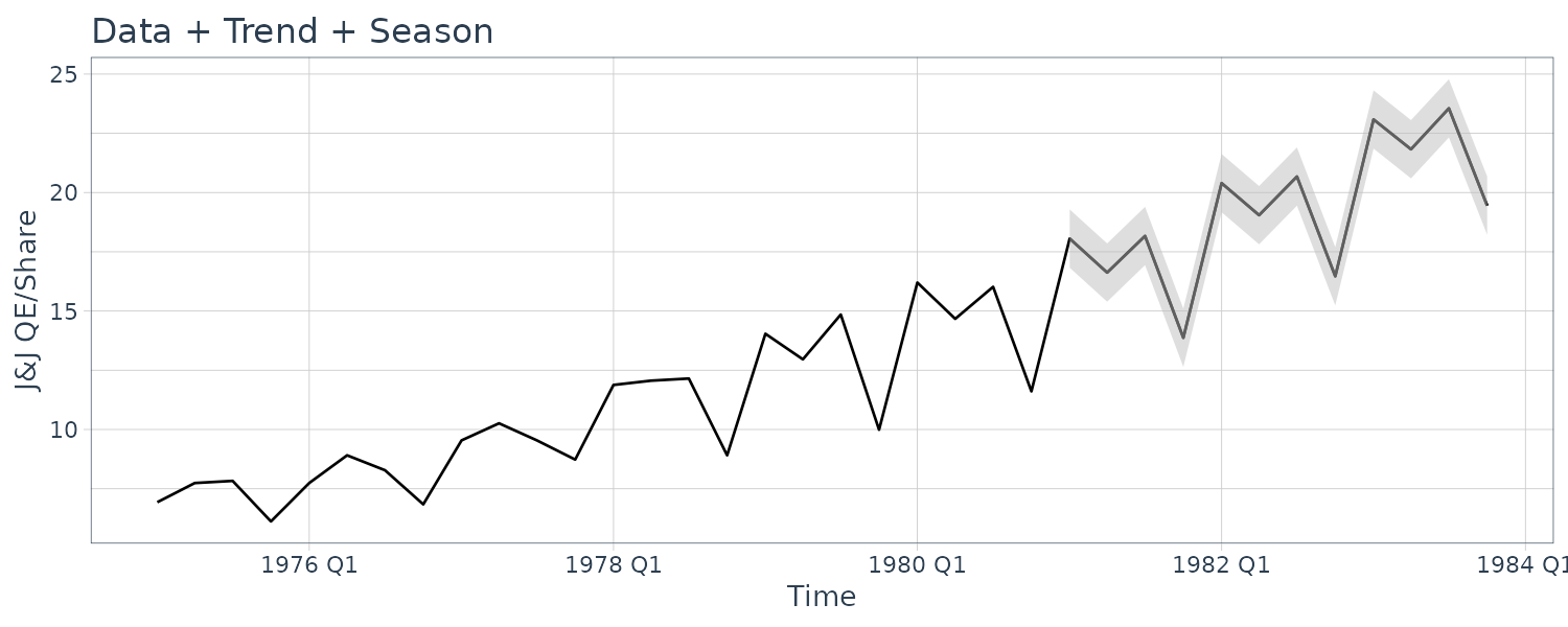

And doing this using dlm package:

set.seed(123)
dat <- as_tsibble(jj)

mod <- dlmModPoly(
  order = 1
) +
  dlmModSeas(
    frequency = 4
  )

mod$m0 <- c(0.7, 0, 0, 0)
mod$GG[1, 1] <- 1.03
mod$C0 <- diag(0.04, 4)
init.par <- c(1.03, 0.1, 0.1, 0.5)

build_dlm <- function(par) {
  mod$W[1, 1] <- exp(par[2])
  mod$W[2, 2] <- exp(par[3])
  mod$V <- exp(par[4])

  mod$GG[1, 1] <- par[1]

  mod
}

fit_dlm <- dlmMLE(
  y = dat$value,
  parm = init.par,
  build = build_dlm,
  hessian = TRUE
)
fit_dlm$par

SEs <- sigmas *
  sqrt(diag(solve(fit_dlm$hessian[2:4, 2:4])))

u <- cbind(
  c(fit_dlm$par[1], sigmas),
  c(sqrt(1 / fit_dlm$hessian[1]), SEs)
)

rownames(u) <- c("Phi11", "sigw1", "sigw2", "sigv")    

> u
              [,1]        [,2]
Phi11 1.0350836112 0.002530973
sigw1 0.1397068026 0.043017970
sigw2 0.2208696600 0.047496915
sigv  0.0001974406 0.003995904

s_var <- dlmSvd2var(
  dlmSmoothed_obj$U.S,
  dlmSmoothed_obj$D.S
) |>
  dropFirst()
s_var <- array(
  unlist(s_var),
  dim = c(4, 4, 84)
)
s_var

dat <- dat |>
  mutate(
    Tsm = dropFirst(dlmSmoothed_obj$s)[, 1],
    Ssm = dropFirst(dlmSmoothed_obj$s)[, 2],
    p1 = 3 * sqrt(s_var[1, 1, ]),
    p2 = 3 * sqrt(s_var[2, 2, ])
  )

And forecasting:

dlmFiltered_obj <- dlmFilter(
  y = dat$value,
  mod = mod
)

nAhead <- 12
dlmForecasted_obj <- dlmForecast(
  mod = dlmFiltered_obj,
  nAhead = nAhead
)

s_var <- array(
  unlist(dlmForecasted_obj$R),
  dim = c(4, 4, nAhead)
)
s_var

dat_pred <- new_data(dat, n = nAhead)
dat_pred <- dat_pred |>
  mutate(
    a = dlmForecasted_obj$a[, 1] +
      dlmForecasted_obj$a[, 2],
    a_sdev = sqrt(
        s_var[1, 1, ] + s_var[2, 2, ]
    ),
    lower = a + qnorm(0.025, sd = a_sdev),    
    upper = a + qnorm(0.975, sd = a_sdev)
  )

Hidden Markov Models

We have been focusing primarily on linear Gaussian state space models, but there is an entire area that has developed around the case where the states \(x_{t}\) are a discrete-valued Markov chain, and that will be the focus in this section. The basic idea is that the value of the state at time t specifies the distribution of the observation at time t.

In the Markov chain approach, we declare the dynamics of the system at time t are generated by one of m possible regimes evolving according to a Markov chain over time. The case in which the particular regime is unknown to the observer comes under the heading of hidden Markov models (HMM).

Although the model satisfies the conditions for being a state space model, HMMs were developed in parallel. If the state process is discrete-valued, one typically uses the term “hidden Markov model” and if the state process is continuous-valued, one uses the term “state space model” or one of its variants.

Here, we assume the states, \(x_{t}\), are a Markov chain taking values in a finite state space \(\{1, \cdots, m\}\), with stationary distribution:

\[\begin{aligned} \pi_{j} &= P(x_{t} = j) \end{aligned}\]

And stationary transition probabilities:

\[\begin{aligned} \pi_{ij} &= P(x_{t+1} = j|x_{t} = i) \end{aligned}\] \[\begin{aligned} t &= 0, 1, 2, \cdots\\ i &= 1, \cdots, m\\ j &= 1, \cdots, m\\ \end{aligned}\]

Since the second component of the model is that the observations are conditionally independent, we need to specify the distributions, and we denote them by:

\[\begin{aligned} P_{j}(y_{t}) &= P(y_{t}|x_{t} = j) \end{aligned}\]

Example: Poisson HMM – Number of Major Earthquakes

Consider the time series of annual counts of major earthquakes. A natural model for unbounded count data is a Poisson distribution, in which case the mean and variance are equal.

However, the sample mean and variance of the data are \(\bar{x} = 19.4\) and \(s^{2} = 51.6\), so this model is clearly inappropriate.

library(astsa)

> mean(EQcount)  
[1] 19.36449

> var(EQcount)
[1] 51.57344

It would be possible to take into account the overdispersion by using other distributions for counts such as the negative binomial distribution or a mixture of Poisson distributions. This approach, however, ignores the sample ACF and PACF which indicate the observations are serially correlated, and further suggest an AR(1)-type correlation structure. A simple and convenient way to capture both the marginal distribution and the serial dependence is to consider a Poisson-HMM model.

Let \(y_{t}\) denote the number of major earthquakes in year t, and consider the state, or latent variable, \(x_{t}\) to be a stationary two-state Markov chain taking values in \(\{1, 2\}\).

We have:

\[\begin{aligned} \pi_{12} &= 1 - \pi_{11}\\ \pi_{21} &= 1 - \pi_{22} \end{aligned}\]

The stationary distribution of this Markov chain is given by:

\[\begin{aligned} \pi_{1} &= \frac{\pi_{21}}{\pi_{12} + \pi_{21}}\\ \pi_{2} &= \frac{\pi_{12}}{\pi_{12} + \pi_{21}} \end{aligned}\]

For \(j \in \{1, 2\}\), denote \(\lambda_{j} > 0\) as the parameter of a Poisson distribution:

\[\begin{aligned} P_{j}(y) &= \frac{\lambda_{j}^{y}e^{-\lambda_{j}}}{y!} \end{aligned}\] \[\begin{aligned} y &= 0, 1, \cdots \end{aligned}\]

Since the states are stationary, the marginal distribution of \(y_{t}\) is stationary and a mixture of Poissons:

\[\begin{aligned} P_{\boldsymbol{\Theta}}(y_{t}) &= \pi_{1}P_{1}(y_{t}) + \pi_{2}P_{2}(y_{t}) \end{aligned}\] \[\begin{aligned} \boldsymbol{\Theta} &= \{\lambda_{1}, \lambda_{2}\} \end{aligned}\]

The mean of the stationary distribution is:

\[\begin{aligned} E[y_{t}] &= \pi_{1}\lambda_{1} + \pi_{2}\lambda_{2} \end{aligned}\]

And the variance is:

\[\begin{aligned} \textrm{var}(y_{t}) &= E[\text{var}(y_{t}|x_{t} = j)] + \text{var}(E[y_{t}|x_{t} = j]) &\geq E[y_{t}] \end{aligned}\]

Similar calculations show that the autocovariance function of yt is given by:

\[\begin{aligned} \gamma_{y}(h) &= \sum_{i=1}^{2}\sum_{j=1}^{2}\pi_{i}(\pi_{ij}^{h} - \pi_{j})\lambda_{i}\lambda_{j}\\ &= \pi_{1}\pi_{2}(\lambda_{2} - \lambda_{1})^{2}(1 - \pi_{12} - \pi_{2})^{h} \end{aligned}\]

Thus, a two-state Poisson-HMM has an exponentially decaying autocorrelation function, and this is consistent with the sample ACF seen in the plot below. It is worthwhile to note that if we increase the number of states, more complex dependence structures may be obtained.

EQcount <- as_tsibble(EQcount)   

EQcount |>
  ACF(value) |>
  autoplot() +
  theme_tq()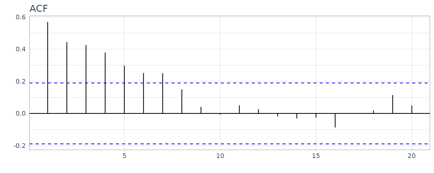

As in the linear Gaussian case, we need filters and smoothers of the state and additionally for estimation and prediction:

\[\begin{aligned} \pi_{j}(t | s) &= P(x_{t} = j | y_{1:s}) \end{aligned}\]

HMM Filter

\[\begin{aligned} \pi_{j}(t | t-1) &= \sum_{i=1}^{m}\pi(t-1|t-1)\pi_{ij}\\ \pi_{j}(t | t) &= \frac{\pi_{j}(t)P_{j}(y_{t})}{\sum_{i=1}^{m}\pi_{i}(t)P_{i}(y_{t})} \end{aligned}\] \[\begin{aligned} t &= 1, \cdots, n \end{aligned}\] \[\begin{aligned} \pi_{j}(1 | 0) &= \pi_{j} \end{aligned}\]

Let \(\boldsymbol{\Theta}\) denote the parameters of interest.

The likelihood is given by:

\[\begin{aligned} L_{Y}(\boldsymbol{\Theta}) &= \prod_{t=1}^{n}P_{\boldsymbol{\Theta}}(y_{t}|y_{1:t-1}) \end{aligned}\]

By the conditional independence:

\[\begin{aligned} P_{\boldsymbol{\Theta}}(y_{t}|y_{1:t-1}) &= \sum_{j=1}^{m}P(x_{t} = j|y_{1:t-1})P_{\boldsymbol{\Theta}}(y_{j}|x_{t} = j, y_{1:t-1})\\ &= \sum_{j=1}^{m}\pi_{j}(t|t-1)P_{j}(y_{t}) \end{aligned}\] \[\begin{aligned} \ln L_{Y}(\boldsymbol{\Theta}) &= \sum_{t=1}^{n}\ln\Big(\sum_{j=1}^{m}\pi_{j}(t|t-1)P_{j}(y_{t})\Big) \end{aligned}\]

Maximum likelihood can then proceed as in the linear Gaussian case. In addition, the EM algorithm applies here as well. First, the general complete data likelihood still has the form of:

\[\begin{aligned} \ln P_{\boldsymbol{\Theta}}(x_{0:n}, y_{1:n}) &= \ln P_{\boldsymbol{\Theta}}(x_{0}) + \sum_{t=1}^{n}\ln P_{\boldsymbol{\Theta}}(x_{t}|x_{t-1}) + \sum_{t=1}^{n}\ln P_{\boldsymbol{\Theta}}(y_{t}|x_{t}) \end{aligned}\]

HMM Smoother

\[\begin{aligned} \pi_{j}(t|n) &= \frac{\pi_{j}(t|t)\varphi_{j}(t)}{\sum_{j=1}^{m}\pi_{j}(t|t)\varphi_{j}(t)}\\ \pi_{ij}(t|n) &= \frac{\pi_{i}(t|n)\pi_{ij}P_{j}(y_{t+1})\varphi_{j}(t+1)}{\varphi_{i}(t)}\\ \end{aligned}\] \[\begin{aligned} t &= n-1, \cdots, 0 \end{aligned}\] \[\begin{aligned} \varphi_{i}(t) &= \sum_{j=1}^{m}\pi_{ij}P_{j}(y_{t+1})\varphi_{j}(t+1) \end{aligned}\]

It is more useful to define \(I_{j}(t) = 1\) if \(x_{t} = j\) and 0 otherwise, and \(I_{ij}(t) = 1\) if \((x_{t−1}, x_{t}) = (i, j)\) and 0 otherwise, for \(i, j = 1, \cdots, m\).

Recall \(P(I_{j}(t) = 1) = \pi_{j}\) and \(P(I_{ij}(t) = 1) = \pi_{ij}\pi_{i}\).

Then the complete data likelihood can be written as:

\[\begin{aligned} \ln P_{\boldsymbol{\Theta}}(x_{0:n}, y_{1:n}) &= \sum_{j=1}^{m}I_{j}(0)\ln\pi_{j} + \sum_{t=1}^{n}\sum_{i=1}^{m}\sum_{j=1}^{m}I_{ij}(t)\ln\pi_{ij}(t) + \sum_{t=1}^{n}\sum_{j=1}^{m}I_{j}(t)\ln P_{j}(y_{t}) \end{aligned}\]

We need to maximize:

\[\begin{aligned} \textbf{W}_{t}(\boldsymbol{\Theta}|\boldsymbol{\Theta}^{T}) &= E[\ln P_{\boldsymbol{\Theta}}(x_{0:n}, y_{1:n})|y_{1:n}, \boldsymbol{\Theta}^{T}] \end{aligned}\]

Example: Poisson HMM – Number of Major Earthquakes

To run the EM algorithm in this case, we still need to maximize the conditional expectation of the third term of:

\[\begin{aligned} \ln P_{\boldsymbol{\Theta}}(x_{0:n}, y_{1:n}) &= \sum_{j=1}^{m}I_{j}(0)\ln\pi_{j} + \sum_{t=1}^{n}\sum_{i=1}^{m}\sum_{j=1}^{m}I_{ij}(t)\ln\pi_{ij}(t) + \sum_{t=1}^{n}\sum_{j=1}^{m}I_{j}(t)\ln P_{j}(y_{t}) \end{aligned}\]

The conditional expectation of the third term at the current parameter value \(\boldsymbol{\Theta}\):

\[\begin{aligned} \sum_{t=1}^{n}\sum_{j=1}^{m}\pi_{j}(t|t-1)\ln P_{j}(y_{t}) \end{aligned}\]

Where:

\[\begin{aligned} \log P_{j}(y_{t}) \propto y_{t}\log \lambda_{j} - \lambda_{j} \end{aligned}\]

Consequently, maximization with respect to \(\lambda_{j}\) yields:

\[\begin{aligned} \hat{\lambda_{j}} &= \frac{\sum_{t=1}^{n}\pi_{j}(t|n)y_{t}}{\sum_{t=1}^{n}\pi_{j}(t|n)} \end{aligned}\] \[\begin{aligned} j &= 1, \cdots, m \end{aligned}\]

We fit the model to the time series of earthquake counts using the R package depmixS4. The package, which uses the EM algorithm, does not provide standard errors, so we obtained them by a parametric bootstrap procedure.

To code this in R:

library(depmixS4)
model <- depmix(
  value ~ 1,
  nstates = 2,
  data = EQcount,
  family = poisson()
)

> model
Initial state probabilities model 
pr1 pr2 
0.5 0.5 

Transition matrix 
       toS1 toS2
fromS1  0.5  0.5
fromS2  0.5  0.5

Response parameters 
Resp 1 : poisson 
    Re1.(Intercept)
St1               0
St2               0

set.seed(90210)
fm <- depmixS4::fit(model)

> summary(fm)
Initial state probabilities model    
pr1 pr2 
  1   0 

Transition matrix 
        toS1  toS2
fromS1 0.928 0.072
fromS2 0.119 0.881

Response parameters 
Resp 1 : poisson 
    Re1.(Intercept)
St1           2.736
St2           3.259

Running the EM algorithm, we see the transition matrix has being updated with the new set of lambdas.

Ignoring the initial state probabilities and retrieving the transition matrix and lambdas:

# estimation results
##-- Get Parameters --##
pars <- getpars(fm)

> pars
        pr1         pr2                                                 
 1.00000000  0.00000000  0.92834885  0.07165115  0.11895483  0.88104517      
(Intercept) (Intercept) 
 2.73560113  3.25865227 

u <- as.vector(pars) # ensure state 1 has smaller lambda

if (u[7] <= u[8]) {
  para.mle <- c(u[3:6], exp(u[7]), exp(u[8]))
} else {
  para.mle <- c(u[6:3], exp(u[8]), exp(u[7]))
}

mtrans <- matrix(
  para.mle[1:4],
  byrow = TRUE,
  nrow = 2
)

lams <- para.mle[5:6]

> lams
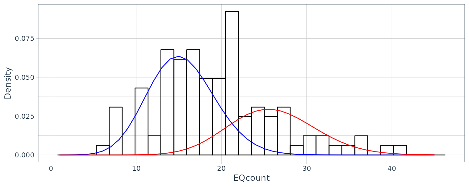
[1] 15.41901 26.01445

The stationary probabilities:

pi1 <- mtrans[2, 1] / (2 - mtrans[1, 1] - mtrans[2, 2])    

> pi1
[1] 0.6240876

pi2 <- 1 - pi1

> pi2
[1] 0.3759124

Retrieving the posterior states and probabilities for each state:

EQcount$state <- posterior(fm)$state
EQcount$S1 <- posterior(fm)$S1
EQcount$S2 <- posterior(fm)$S2

dat <- tibble(
  xvals = seq(1, 45),
  u1 = pi1 * dpois(xvals, lams[1]),
  u2 = pi2 * dpois(xvals, lams[2])
)

Plotting:

EQcount |>
  ggplot(aes(x = index, y = value)) +
  geom_segment(
    aes(x = index, xend = index, y = 0, yend = value),      
    alpha = 0.5
  ) +
  geom_text(
    aes(
      y = value + 1,
      label = state,
      col = factor(state)
    ),
    hjust = 1
  ) +
  xlab("") +
  ylab("EQcount") +
  theme_tq()

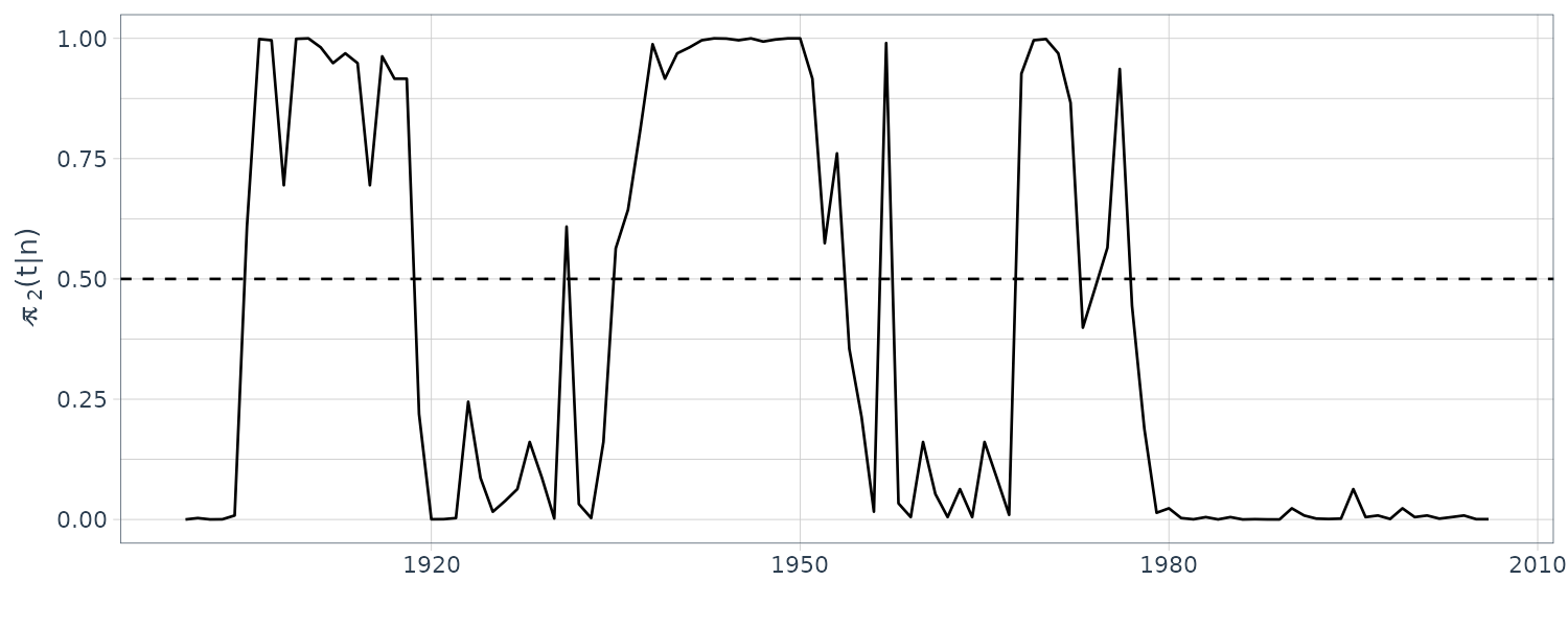
EQcount |>
  autoplot(S2) +
  xlab("") +
  ylab(expression(hat(pi)[~2] * "(t|n)")) +
  geom_hline(yintercept = 0.5, linetype = "dashed") +    
  theme_tq()

EQcount |>
  ggplot(aes(x = value)) +
  geom_histogram(
    aes(y = ..density..),
    fill = "transparent",
    col = "black"
  ) +
  geom_line(
    aes(x = xvals, y = u1),
    data = dat,
    col = "blue"
  ) +
  geom_line(
    aes(x = xvals, y = u2),
    data = dat,
    col = "red"
  ) +
  ylab("Density") +
  xlab("EQcount") +
  theme_tq()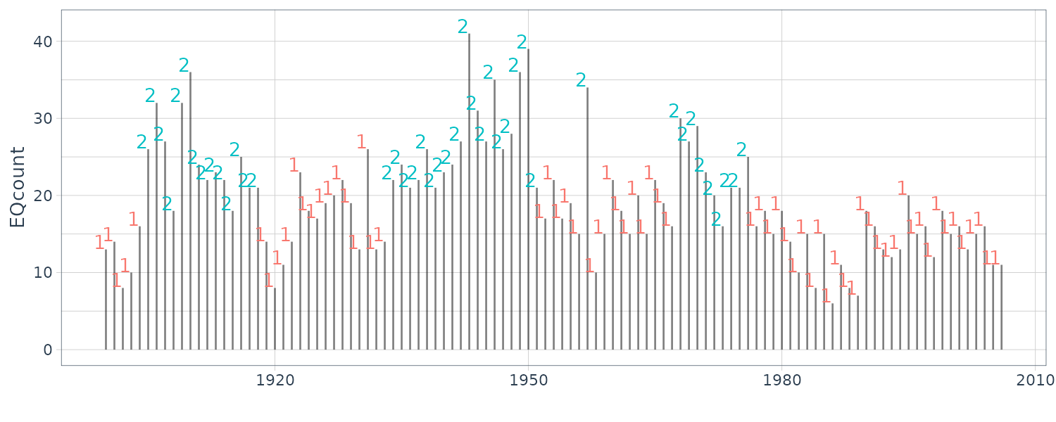

The package, which uses the EM algorithm, does not provide standard errors, so we obtained them by a parametric bootstrap procedure:

pois.HMM.generate_sample <-
  function(n, m, lambda, Mtrans, StatDist = NULL) {
    if (is.null(StatDist)) {
      StatDist <- solve(
        t(diag(m) - Mtrans + 1),
        rep(1, m)
      )
    }

    mvect <- 1:m
    state <- numeric(n)
    state[1] <- sample(mvect, 1, prob = StatDist)

    for (i in 2:n) {
      state[i] <- sample(mvect, 1, prob = Mtrans[state[i - 1], ])      
    }

    y <- rpois(n, lambda = lambda[state])

    list(
      y = y,
      state = state
    )
  }

# start it up
set.seed(10101101)
nboot <- 100
nobs <- nrow(EQcount)
para.star = matrix(NA, nrow = nboot, ncol = 6)

for (j in 1:nboot) {
  x.star = pois.HMM.generate_sample(
    n = nobs,
    m = 2,
    lambda = lams,
    Mtrans = mtrans
  )$y

  model <- depmix(
    x.star ~ 1,
    nstates = 2,
    data = data.frame(x.star),
    family = poisson()
  )

  u <- as.vector(
    getpars(
      depmixS4::fit(model, verbose = 0)
    )
  )

  # make sure state 1 is the one with the smaller
  # intensity parameter
  if (u[7] <= u[8]) {
    para.star[j, ] = c(u[3:6], exp(u[7]), exp(u[8]))
  } else {
    para.star[j, ] = c(u[6:3], exp(u[8]), exp(u[7]))
  }
}

# bootstrapped std errors
SE <- sqrt(apply(para.star, 2, var) +
  (apply(para.star, 2, mean) - para.mle)^2)[c(1, 4:6)]
names(SE) <- c("seM11/M12", "seM21/M22", "seLam1", "seLam2")     

> SE
 seM11/M12  seM21/M22     seLam1     seLam2 
0.04074297 0.09218465 0.66300322 1.10658114 

Example: Normal HMM – S&P500 Weekly Returns

Estimation in the Gaussian case is similar to the Poisson case except that now, \(p_{j}(y_{t})\) is the normal density:

\[\begin{aligned} (y_{t} | x_{t} = j) &\sim N(\mu_{j}, \sigma_{j}^{2}) \end{aligned}\] \[\begin{aligned} j &= 1, \cdots, m \end{aligned}\]

Then dealing with the third term in:

\[\begin{aligned} \ln P_{\boldsymbol{\Theta}}(x_{0:n}, y_{1:n}) &= \sum_{j=1}^{m}I_{j}(0)\ln\pi_{j} + \sum_{t=1}^{n}\sum_{i=1}^{m}\sum_{j=1}^{m}I_{ij}(t)\ln\pi_{ij}(t) + \sum_{t=1}^{n}\sum_{j=1}^{m}I_{j}(t)\ln P_{j}(y_{t}) \end{aligned}\]

Yields:

\[\begin{aligned} \hat{\mu}_{j} &= \frac{\sum_{t=1}^{n}\pi_{j}(tn)y_{t}}{\sum_{t=1}^{n}\pi_{j}(t|n)}\\ \hat{\sigma}_{j}^{2} &= \frac{\sum_{t=1}^{n}\pi_{j}(tn)y_{t}^{2}}{\sum_{t=1}^{n}\pi_{j}(t|n)} - \hat{\mu}_{j}^{2}\\ \end{aligned}\]

In this example, we fit a normal HMM using the R package depmixS4 to the weekly S&P 500 returns. We chose a three-state model.

The data, along with the predicted state:

dat <- tsibble(
  t = seq(
    as.Date("2003-01-01"),
    as.Date("2012-10-01"),
    by = "1 week"
  ) |>
    yearweek(),
  y = as.vector(sp500w),
  index = t
)

mod3 <- depmix(
  y ~ 1,
  nstates = 3,
  data = dat
)
set.seed(2)
fm3 <- depmixS4::fit(mod3)

> summary(fm3)
summary(fm3)
Initial state probabilities model 
pr1 pr2 pr3 
  1   0   0 

Transition matrix 
        toS1  toS2  toS3
fromS1 0.942 0.027 0.032
fromS2 0.261 0.000 0.739
fromS3 0.000 0.055 0.945

Response parameters 
Resp 1 : gaussian 
    Re1.(Intercept) Re1.sd
St1          -0.003  0.044
St2          -0.034  0.009
St3           0.004  0.014

dat$state <- posterior(fm3)$state    
dat$S1 <- posterior(fm3)$S1
dat$S2 <- posterior(fm3)$S2
dat$S3 <- posterior(fm3)$S3

dat |>
  autoplot(y, alpha = 0.2) +
  geom_text(
    aes(
      y = y + 0.03,
      label = state,
      col = factor(state)
    ),
    hjust = 1
  ) +
  xlab("") +
  ylab("S&P 500 Weekly Returns") +    
  theme_tq() +
  theme(legend.position = "none")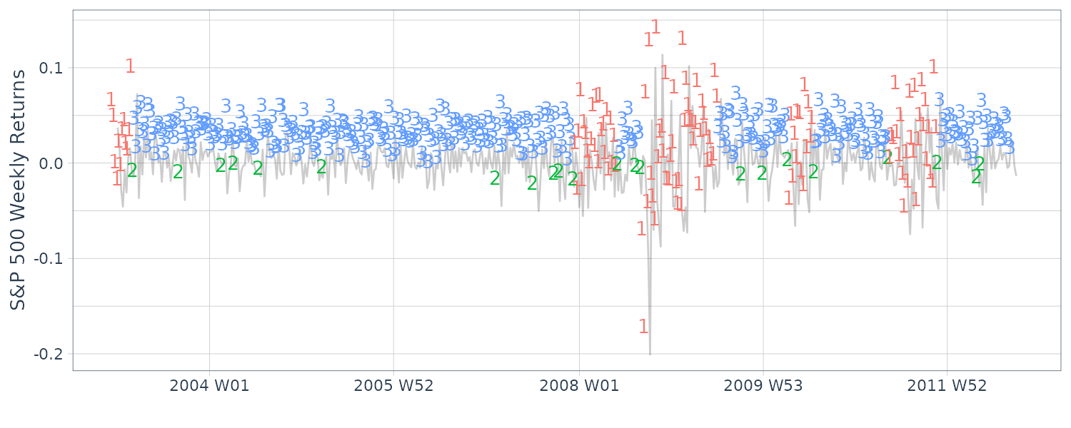

The fitted transition matrix:

\[\begin{aligned} \hat{P} &= \begin{bmatrix} 0.942 & 0.032 & 0.027\\ 0.261 & 0.000 & 0.739\\ 0.032 & 0.055 & 0.945\\ \end{bmatrix} \end{aligned}\]

And the 3 fitted normals distribution:

\[\begin{aligned} N(\hat{\mu}_{1} = -0.003, \hat{\sigma}_{1} = 0.044)\\ N(\hat{\mu}_{2} = -0.034, \hat{\sigma}_{2} = 0.009)\\ N(\hat{\mu}_{3} = 0.004, \hat{\sigma}_{3} = 0.014)\\ \end{aligned}\]

Computing the transition matrix in R:

mtrans.mle <- as.vector(
  getpars(fm3)[-(1:3)]
)

> round(
  matrix(para.mle[1:9], 3, 3),    
  3
)
      [,1]  [,2]  [,3]
[1,] 0.942 0.261 0.000
[2,] 0.027 0.000 0.055
[3,] 0.032 0.739 0.945

And for the means and standard deviations of the normal distributions. The first row are the means and second row the standard deviations:

norms.mle <- round(
  matrix(para.mle[10:15], 2, 3),    
  3
)

> norms.mle
[1,] -0.003 -0.034 0.004
[2,]  0.044  0.009 0.014

Note that regime 2 appears to represent a somewhat large-in-magnitude negative return, and may be a lone dip, or the start or end of a highly volatile period.

States 3 and 1 represent clusters of regular or high volatility, respectively. Note that there is a large amount of uncertainty in the fitted normals, and in the transition matrix involving transitions from state 2 to states 1 or 3.

Graphing the histogram and the 3 estimated normal densities superimposed and scaled by the posterior probabilities:

dat2 <- tibble(
  x = seq(-.15, .12, by = .001),
  u1 = pi.hat[1] *
    dnorm(
      x,
      mean = norms.mle[1, 1],
      sd = norms.mle[2, 1]
    ),
  u2 = pi.hat[2] *
    dnorm(
      x,
      mean = norms.mle[1, 2],
      sd = norms.mle[2, 2]
    ),
  u3 = pi.hat[3] *
    dnorm(
      x,
      mean = norms.mle[1, 3],
      sd = norms.mle[2, 3]
    )
)

dat3 <- gather(
  dat2,
  State,
  y2,
  u1,
  u2,
  u3
)

dat |>
  ggplot(aes(x = y)) +
  geom_histogram(
    aes(y = ..density..),
    fill = "transparent",
    col = "black"
  ) +
  geom_line(
    aes(x = x, y = y2, col = State),
    data = dat3
  ) +
  ylab("Density") +
  xlab("") +
  theme_tq()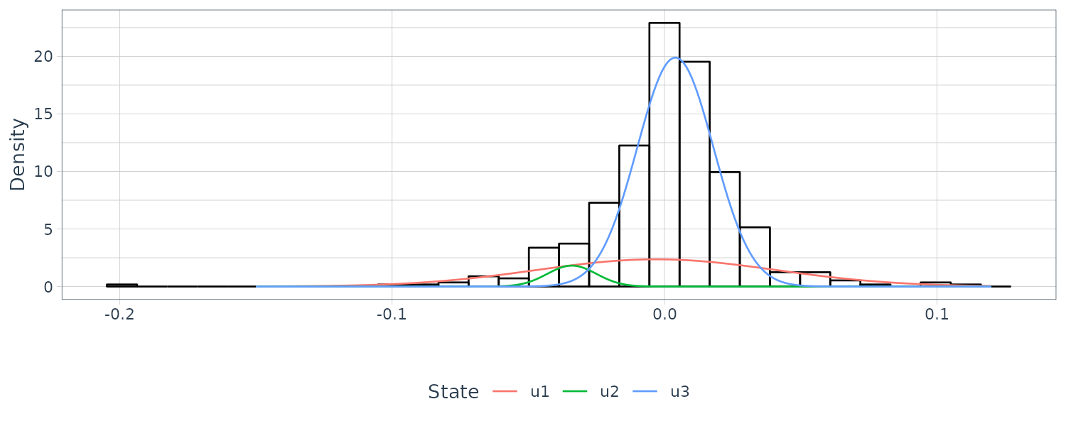

Bootstrapping the standard errors:

set.seed(666)
n.obs <- length(y)
n.boot <- 100
para.star <- matrix(NA, nrow = n.boot, ncol = 15)
respst <- para.mle[10:15]
trst <- para.mle[1:9]

for (nb in 1:n.boot) {
  mod <- depmixS4::simulate(mod3)

  y.star <- as.vector(mod@response[[1]][[1]]@y)
  dfy <- data.frame(y.star)

  mod.star <- depmix(
    y.star ~ 1,
    data = dfy,
    respst = respst,
    trst = trst,
    nst = 3
  )

  fm.star <- depmixS4::fit(
    mod.star,
    emcontrol = em.control(tol = 1e-5),
    verbose = FALSE
  )
  para.star[nb, ] <- as.vector(getpars(fm.star)[-(1:3)])    
}

SE <- sqrt(
  apply(para.star, 2, var) +
    (apply(para.star, 2, mean) - para.mle)^2
)

SE.mtrans.mle <- round(matrix(SE[1:9], 3, 3), 3)

> SE.mtrans.mle
       [,1]  [,2]  [,3]
[1,] 0.147 0.275 0.000
[2,] 0.057 0.000 0.074
[3,] 0.122 0.275 0.074

SE.norms.mle <- round(matrix(SE[10:15], 2, 3), 3)

> SE.norms.mle
       [,1]  [,2]  [,3]
[1,] 0.317 0.909 0.173
[2,] 0.910 0.777 0.968

Switching AR – Influenza Mortality

Note that the series is irregular, and while mortality is highest during the winter, the peak does not occur in the same month each year. Moreover, some seasons have very large peaks, indicating flu epidemics, whereas other seasons are mild. In addition, it can be seen that there is a slight negative trend in the data set, indicating that flu prevention is getting better over the eleven year period.

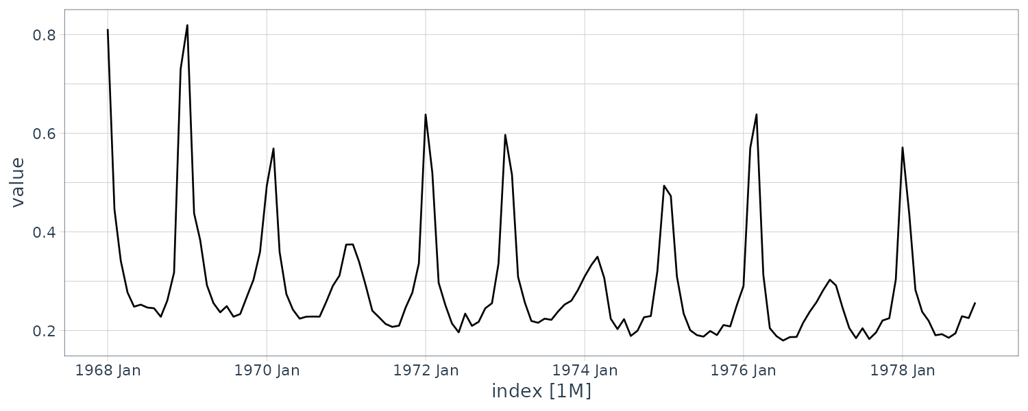
We focus on the differenced data, which removes the trend. In this case, we denote \(y_{t} = \nabla flu_{t}\). Since we already fit a threshold model to \(y_{t}\), we might also consider a switching autoregressive model where there are two hidden regimes, one for epidemic periods and one for more mild periods. In this case, the model is given by:

\[\begin{aligned} y_{t} &= \begin{cases} \phi_{0}^{(1)} + \sum_{j=1}^{p}\phi_{j}^{(1)}y_{t-j} + \sigma^{(1)}v_{t} & x_{t} = 1\\ \phi_{0}^{(2)} + \sum_{j=1}^{p}\phi_{j}^{(2)}y_{t-j} + \sigma^{(2)}v_{t} & x_{t} = 2\\ \end{cases} \end{aligned}\] \[\begin{aligned} v_{t} &\sim N(0, 1) \end{aligned}\]

And \(x_{t}\) is a latent, two-state Markov chain.

We used the R package MSwM to fit the model with p = 2:

\[\begin{aligned} y_{t} &= \begin{cases} 0.006 + 0.293 y_{t-1} + 0.097 y_{t-2} + 0.021 v_{t} & x_{t} = 1\\ 0.199 - 0.313 y_{t-1} - 1.604 y_{t-2} + 0.112 v_{t} & x_{t} = 2 \end{cases} \end{aligned}\]

With estimated transition matrix:

\[\begin{aligned} \hat{P} &= \begin{bmatrix} 0.93 & 0.07\\ 0.30 & 0.70 \end{bmatrix} \end{aligned}\]

Doing this in R:

set.seed(90210)

model <- lm(dflu ~ 1, data = flu)   
mod <- msmFit(
  model,
  k = 2,
  p = 2,
  sw = rep(TRUE, 4)
)

> summary(mod)
Markov Switching Model

Call: msmFit(object = model, k = 2, sw = rep(TRUE, 4), p = 2)

        AIC       BIC   logLik
  -438.6622 -392.3445 225.3311

Coefficients:

Regime 1 
---------
               Estimate Std. Error t value       Pr(>|t|)    
(Intercept)(S)   0.1989     0.0629  3.1622       0.001566 ** 
dflu_1(S)       -0.3127     0.2805 -1.1148       0.264936    
dflu_2(S)       -1.6042     0.2762 -5.8081 0.000000006319 ***
---
Signif. codes:  0 ‘***’ 0.001 ‘**’ 0.01 ‘*’ 0.05 ‘.’ 0.1 ‘ ’ 1

Residual standard error: 0.1120415
Multiple R-squared: 0.6939

Standardized Residuals:
         Min           Q1          Med           Q3          Max 
-0.170236363 -0.014869233 -0.007706104 -0.003753905  0.284000551 

Regime 2 
---------
               Estimate Std. Error t value            Pr(>|t|)    
(Intercept)(S)   0.0058     0.0027  2.1481            0.031706 *  
dflu_1(S)        0.2931     0.0392  7.4770 0.00000000000007594 ***     
dflu_2(S)        0.0970     0.0312  3.1090            0.001877 ** 
---
Signif. codes:  0 ‘***’ 0.001 ‘**’ 0.01 ‘*’ 0.05 ‘.’ 0.1 ‘ ’ 1

Residual standard error: 0.02359005
Multiple R-squared: 0.497

Standardized Residuals:
                 Min                   Q1                  Med
-0.07374090551591896 -0.00801780462200020  0.00000000001010047
                  Q3                  Max 
0.01230736214172173  0.04700877108891068 

Transition probabilities:
          Regime 1   Regime 2
Regime 1 0.7004731 0.07335256
Regime 2 0.2995269 0.92664744

plotProb(mod, which = 3)

Dynamic Linear Models with Switching

In this section, we extend the hidden Markov model to more general problems. Generalizations of the state space model to include the possibility of changes occurring over time have been approached by allowing changes in the error covariances or by assigning mixture distributions to the observation errors \(v_{t}\).

One way of modeling change in an evolving time series is by assuming the dynamics of some underlying model changes discontinuously at certain undetermined points in time. Our starting point is the DLM:

\[\begin{aligned} x_{t} &= \textbf{G}_{t} x_{t-1} + w_{t} \end{aligned}\]

To describe the p x 1 state dynamics and:

\[\begin{aligned} y_{t} &= \textbf{F}_{t}x_{t} + v_{t} \end{aligned}\]

To describe the q × 1 observation dynamics. Recall \(w_{t}\) and \(v_{t}\) are Gaussian white noise sequences with \(\textrm{var}(w_{t}) = \textbf{W}_{t}\), \(\textrm{var}(v_{t}) = \textbf{V}_{t}\), and \(\textrm{cov}(w_{t}, v_{s}) = 0\) for all s and t.

Example: Tracking Multiple Targets

The approach was motivated primarily by the problem of tracking a large number of moving targets using a vector \(y_{t}\) of sensors. In this problem, we do not know at any given point in time which target any given sensor has detected. Hence, it is the structure of the measurement matrix \(\textbf{F}_{t}\) that is changing, and not the dynamics of the signal \(x_{t}\) or the noises, \(w_{t}\) or \(v_{t}\). As an example, consider a 3 × 1 vector of satellite measurements \(\textbf{y}_{t} = (y_{t1}, y_{t2}, y_{t3})\) that are observations on some combination of a 3 × 1 vector of targets or signals, \(\textbf{x}_{t} = (x_{t1}, x_{t2}, x_{t3})\). For the measurement matrix:

\[\begin{aligned} \textbf{F}_{t} &= \begin{bmatrix} 0 & 1 & 0\\ 1 & 0 & 0\\ 0 & 0 & 1 \end{bmatrix} \end{aligned}\]

For example, the first sensor, \(y_{t1}\), observes the second target, \(x_{t2}\); the second sensor, \(y_{t2}\), observes the first target, \(x_{t1}\); and the third sensor, \(y_{t3}\), observes the third target, \(x_{t3}\). All possible detection configurations will define a set of possible values for \(\textbf{F}_{t}\), say, \(\{M_{1}, M_{2}, \cdots, M_{m}\}\), as a collection of plausible measurement matrices.

Modeling Economic Change

As another example of the switching model presented in this section, consider the case in which the dynamics of the linear model changes suddenly over the history of a given realization. For example, given the following generalization of model for detecting positive and negative growth periods in the economy. Suppose the data are generated by:

\[\begin{aligned} y_{t} &= z_{t} + n_{t} \end{aligned}\]

Where \(z_{t}\) is an autoregressive series and \(n_{t}\) is a random walk with a drift that switches between two values \(\alpha_{0}\) and \(\alpha_{0} + \alpha_{1}\). That is:

\[\begin{aligned} n_{t}&= n_{t-1} + \alpha_{0} + \alpha_{1}S_{t} \end{aligned}\]

With \(S_{t} = 0\) or \(S_{t} = 1\), depending on whether the system is in state 1 or state 2. For the purpose of illustration, suppose:

\[\begin{aligned} z_{t} &= \phi_{1}z_{t-1} + \phi_{2}z_{t-2} + w_{t} \end{aligned}\]

Is an AR(2) series with \(\textrm{var}(w_{t}) = \sigma_{w}^{2}\). In a differenced form:

\[\begin{aligned} \nabla y_{t} &= z_{t} - z_{t-1} + n_{t} - n_{t-1}\\ &= z_{t}- z_{t-1} + \alpha_{0} + \alpha_{1}S_{t}\\ \end{aligned}\]

With state vector:

\[\begin{aligned} \textbf{x}_{t} &= \begin{bmatrix} z_{t}\\ z_{t-1}\\ \alpha_{0}\\ \alpha_{1} \end{bmatrix} \end{aligned}\]

And determining the two possible economic conditions:

\[\begin{aligned} M_{1} &= [1, -1, 1, 0]\\ M_{2} &= [1, -1, 1, 1] \end{aligned}\]

The state equation is of the form:

\[\begin{aligned} \begin{bmatrix} z_{t}\\ z_{t-1}\\ \alpha_{0}\\ \alpha_{1} \end{bmatrix} &= \begin{bmatrix} \phi_{1} & \phi_{2} & 0 & 0\\ 1 & 0 & 0 & 0\\ 0 & 0 & 1 & 0\\ 0 & 0 & 0 & 1 \end{bmatrix} \begin{bmatrix} z_{t-1}\\ z_{t-2}\\ \alpha_{0}\\ \alpha_{1} \end{bmatrix} + \begin{bmatrix} w_{t}\\ 0\\ 0\\ 0 \end{bmatrix} \end{aligned}\] \[\begin{aligned} \textbf{x}_{t} &= \textbf{G}_{t} \textbf{x}_{t-1} + \textbf{w}_{t} \end{aligned}\]

The observation equation can be written as:

\[\begin{aligned} \nabla \textbf{y}_{t} &= \begin{bmatrix} 1 & -1 & 1 & 1/0 \end{bmatrix} \begin{bmatrix} z_{t-1}\\ z_{t-2}\\ \alpha_{0}\\ \alpha_{1} \end{bmatrix} + \begin{bmatrix} v_{t}\\ 0\\ 0\\ 0 \end{bmatrix}\\ &= \textbf{F}_{t}\textbf{x}_{t} + \textbf{v}_{t} \end{aligned}\]

Where we have included the possibility of observational noise, and where:

\[\begin{aligned} P(\textbf{F}_{t} = M_{1}) &= 1 - P(\textbf{F}_{t} = M_{2}) \end{aligned}\]

To incorporate a reasonable switching structure for the measurement matrix into the DLM that is compatible with both practical situations previously described, we assume that the m possible configurations are states in a nonstationary, independent process defined by the time-varying probabilities:

\[\begin{aligned} \pi_{j}(t) &= P(\textbf{F}_{t} = M_{j}) \end{aligned}\] \[\begin{aligned} j &= 1, \cdots, m\\ t &= 1, 2, \cdots, n \end{aligned}\]

Important information about the current state of the measurement process is given by the filtered probabilities of being in state j, defined as the conditional probabilities:

\[\begin{aligned} \pi_{j}(t | t) &= P(\textbf{F}_{t} = M_{j}|y_{1:t}) \end{aligned}\]

Which also vary as a function of time.

The filtered probabilities give the time-varying estimates of the probability of being in state j given the data to time t.

It will be important for us to obtain estimators of the configuration probabilities, \(\pi_{j}(t \mid t)\), the predicted and filtered state estimators, \(x_{t}^{t−1}\) and \(x_{t}^{t}\), and the corresponding error covariance matrices \(P_{t}^{t−1}\) and \(P_{t}^{t}\). Of course, the predictor and filter estimators will depend on the parameters, \(\boldsymbol{\Theta}\), of the DLM. In many situations, the parameters will be unknown and we will have to estimate them. Our focus will be on maximum likelihood estimation, but we could have taken a Bayesian approach that assigns priors to the parameters, and then seeks posterior distributions of the model parameters.

We now establish the recursions for the filters associated with the state \(x_{t}\) and the switching process, \(\textbf{F}_{t}\). As discussed previously, the filters are also an essential part of the maximum likelihood procedure. The predictors, \(x_{t}^{t−1} = E(x_{t} \mid y_{1:t−1})\), and filters, \(x_{t}^{t} = E(x_{t} \mid y_{1:t})\), and their associated error variance–covariance matrices, \(P_{t}^{t−1}\) and \(P_{t}^{t}\), are given by:

\[\begin{aligned} x_{t}^{t-1} &= \textbf{G}_{t} x_{t-1}^{t-1}\\ P_{t}^{t-1} &= \textbf{G}_{t} P_{t-1}^{t-1}\textbf{G}_{t}^{T} + \textbf{W}_{t} \end{aligned}\] \[\begin{aligned} x_{t}^{t} &= x_{t}^{t-1} + \sum_{j=1}^{m}\pi_{j}(t|t)\textbf{K}_{tj}e_{tj}\\ P_{t}^{t}&= \sum_{j=1}^{m}\pi_{j}(t|t)(\textbf{I} - \textbf{K}_{tj}M_{j})P_{t}^{t-1} \end{aligned}\] \[\begin{aligned} \textbf{K}_{tj} &= P_{t}^{t-1}M_{j}^{T}\textbf{C}_{tj}^{-1}\\ e_{tj} &= y_{t} - M_{j}x_{t}^{t-1}\\ \textbf{C}_{tj} &= M_{j}P_{t}^{t-1}M_{j}^{T} + \textbf{V}_{t} \end{aligned}\] \[\begin{aligned} j &= 1, \cdots, m \end{aligned}\]

Next, we derive the filters \(\pi_{j}(t\mid t)\). Let \(p_{j}(t \mid t − 1)\) denote the conditional density of \(y_{t}\) given the past \(y_{1:t−1}\), and \(\textbf{F}_{t} = M_{j}\), for \(j = 1, \cdots, m\). Then:

\[\begin{aligned} \pi_{j}(t|t) &= \frac{\pi_{j}(t)P_{j}(t|t-1)}{\sum_{k=1}^{m}\pi_{k}(t)P_{k}(t|t-1)} \end{aligned}\]

Where we assume the distribution \(\pi_{j}(t)\), for \(j=1, \cdots, m\) has been specified before observing \(y_{1:t}\).

If the investigator has no reason to prefer one state over another at time t, the choice of uniform priors:

\[\begin{aligned} \pi_{j}(t) = \frac{1}{m} \end{aligned}\]

Example: Hidden Markov Chain Model

If \(\{\textbf{F}_{t}\}\) is a hidden Markov chain with stationary transition probabilities , for i, j = 1, . . . , m, we have

\[\begin{aligned} \pi_{ij} = P(\textbf{F}_{t} = M_{j} | \textbf{F}_{t-1} = Mi) \end{aligned}\] \[\begin{aligned} i &= 1, \cdots, m\\ j &= 1, \cdots, m\\ \end{aligned}\] \[\begin{aligned} \pi_{j}(t|t) &= \frac{P(\textbf{F}_{t} = M_{j}, y_{t}|y_{1:t-1})}{P(y_{t}|y_{1:t-1})}\\ &= \frac{P(\textbf{F}_{t} = M_{j}|y_{1:t-1})P(y_{t}|\textbf{F}_{t} = M_{j}, y_{1:t-1})}{P(y_{t}|y_{1:t-1})}\\ &= \frac{\pi_{j}(t|t-1)P_{j}(t|t-1)}{\sum_{k=1}^{m}\pi_{k}(t|t-1)P_{k}(t|t-1)} \end{aligned}\]

In the Markov case, the condition probabilities:

\[\begin{aligned} \pi_{j}(t|t-1) = P(\textbf{F}_{t} = M_{j}|y_{1:t-1}) \end{aligned}\]

Replace the unconditional probabilities \(\pi_{j}(t) = P(\textbf{F}_{t} = M_{j})\) with \(\pi_{j}(t\mid t-1)\) in:

\[\begin{aligned} \pi_{j}(t|t) &= \frac{\pi_{j}(t)P_{j}(t|t-1)}{\sum_{k=1}^{m}\pi_{k}(t)P_{k}(t|t-1)} \end{aligned}\]

The difficulty in extending the approach here to the Markov case is the dependence among the \(y_{t}\), which makes it necessary to enumerate over all possible histories to derive the filtering equations. This problem will be evident when we derive the conditional density \(P_{j}(t \mid t − 1)\). The below equation:

\[\begin{aligned} \pi_{j}(t) &= \sum_{i=1}^{m}\pi_{i}(t-1|t-1)\pi_{ij} \end{aligned}\]

Has \(\pi_{j}(t)\) as a function of the past observations, \(y_{1:t−1}\), which is inconsistent with our model assumption. Nevertheless, this seems to be a reasonable compromise that allows the data to modify the probabilities \(\pi_{j}(t)\), without having to develop a highly computer-intensive technique.

Example: Analysis of the Influenza Data

We use the results of this section to analyze the U.S. monthly pneumonia and influenza mortality data. Letting \(y_{t}\) denote the observations at month t, we model \(y_{t}\) in terms of a structural component model coupled with a hidden Markov process that determines whether a flu epidemic exists.

The model consists of three structural components. The first component, \(x_{t1}\), is an AR(2) process chosen to represent the periodic (seasonal) component of the data:

\[\begin{aligned} x_{t1} &= \alpha_{1}x_{t-1, 1} + \alpha_{2}x_{t-2,1} + w_{t1} \end{aligned}\] \[\begin{aligned} \textrm{var}(w_{t1}) = \sigma_{1}^{2} \end{aligned}\]

The second component, \(x_{t2}\), is an AR(1) process with a nonzero constant term, which is chosen to represent the sharp rise in the data during an epidemic:

\[\begin{aligned} x_{t2} &= \beta_{0} + \beta_{1}x_{t-1,2} + w_{t2} \end{aligned}\] \[\begin{aligned} \textrm{var}(w_{t2}) = \sigma_{2}^{2} \end{aligned}\]

The third component, \(x_{t3}\) is a fixed trend component given by:

\[\begin{aligned} x_{t3} &= x_{t-1, 3} + w_{t3} \end{aligned}\] \[\begin{aligned} \textrm{var}(w_{t3}) = 0 \end{aligned}\]

The case in which \(\textrm{var}(w_{t3}) > 0\), which corresponds to a stochastic trend (random walk), was tried here, but the estimation became unstable, and lead to us fitting a fixed, rather than stochastic, trend. Thus, in the final model, the trend component satisfies \(\nabla x_{t3} = 0\); recall in previous example the data were also differenced once before fitting the model.

Throughout the years, periods of normal influenza mortality (state 1) are modeled as:

\[\begin{aligned} y_{t} &= x_{t1} + x_{t3} + v_{t} \end{aligned}\]

Where the measurement error, \(v_{t}\) is white noise with \(\textrm{var}(v_{t}) = \sigma_{v}^{2}\). When an epidemic occurs (state 2), mortality is modeled as:

\[\begin{aligned} y_{t} &= x_{t1} + x_{t2} + x_{t3} + v_{t} \end{aligned}\]

The state equation can be written in the general state-space form using the above defined relationships:

\[\begin{aligned} \begin{bmatrix} x_{t1}\\ x_{t-1,1}\\ x_{t2}\\ x_{t3} \end{bmatrix} &= \begin{bmatrix} \alpha_{1} & \alpha_{1} & 0 & 0\\ 1 & 0 & 0 & 0\\ 0 & 0 & \beta_{1} & 0\\ 0 & 0 & 0 & 1\\ \end{bmatrix} \begin{bmatrix} x_{t-1, 1}\\ x_{t-2, 1}\\ x_{t-1, 2}\\ x_{t-1, 3}\\ \end{bmatrix} + \begin{bmatrix} 0\\ 0\\ \beta_{0}\\ 0 \end{bmatrix} + \begin{bmatrix} w_{t1}\\ 0\\ w_{t2}\\ 0 \end{bmatrix} \end{aligned}\]

Or written in the standard state-equation form:

\[\begin{aligned} \textbf{x}_{t} &= \textbf{G}_{t} \textbf{x}_{t-1} + \Psi\textbf{u}_{t} + \textbf{w}_{t} \end{aligned}\] \[\begin{aligned} \textbf{x}_{t} &= \begin{bmatrix} x_{t1}\\ x_{t-1, 1}\\ x_{t2}\\ x_{t3}\\ \end{bmatrix}\\ \Psi &= \begin{bmatrix} 0\\ 0\\ \beta_{0}\\ 0 \end{bmatrix}\\ \textbf{u}_{t} &\equiv 1\\ \textbf{W}_{t} &= \begin{bmatrix} \sigma_{1}^{2} & 0 & 0 & 0\\ 0 & 0 & 0 & 0\\ 0 & 0 & \sigma_{2} & 0\\ 0 & 0 & 0 & 0 \end{bmatrix} \end{aligned}\]

The observation equation is:

\[\begin{aligned} \textbf{y}_{t} &= \textbf{F}_{t}\textbf{x}_{t} + \textbf{v}_{t} \end{aligned}\] \[\begin{aligned} \textrm{var}(\textbf{v}_{t}) &= \textbf{V}_{t}\\ &= \sigma_{v}^{2} \end{aligned}\]

\(\textbf{F}_{t}\) can take one of two possible forms. No epidemic:

\[\begin{aligned} \textbf{F}_{t} &= M_{1}\\ &= [1, 0, 0, 1] \end{aligned}\]

And epidemic:

\[\begin{aligned} \textbf{F}_{t} &= M_{2}\\ &= [1, 0, 1, 1] \end{aligned}\]

Corresponding to the two possible states of (1) no flu epidemic and (2) flu epidemic, such that:

\[\begin{aligned} P(\textbf{F}_{t} = M1) &= 1 - P(\textbf{F}_{t} = M_{2}) \end{aligned}\]

In this example, we will assume \(\textbf{F}_{t}\) is a hidden Markov chain, and hence we use the updating equations:

\[\begin{aligned} \pi_{j}(t|t) &= \frac{P(\textbf{F}_{t} = M_{j}, y_{t}|y_{1:t-1})}{P(y_{t}|y_{1:t-1})}\\ &= \frac{P(\textbf{F}_{t} = M_{j}|y_{1:t-1})P(y_{t}|\textbf{F}_{t} = M_{j}, y_{1:t-1})}{P(y_{t}|y_{1:t-1})}\\ &= \frac{\pi_{j}(t|t-1)P_{j}(t|t-1)}{\sum_{k=1}^{m}\pi_{k}(t|t-1)P_{k}(t|t-1)} \end{aligned}\]

With transition probabilities:

\[\begin{aligned} \pi_{12} &= \pi_{22}\\ &= 0.75 \end{aligned}\]

And thus:

\[\begin{aligned} \pi_{12} &= \pi_{21}\\ &= 0.25 \end{aligned}\]

Parameter estimation was accomplished using a quasi-Newton–Raphson procedure to maximize the approximate log likelihood:

\[\begin{aligned} \ln L_{Y}(\boldsymbol{\Theta}) &= \sum_{t=1}^{n}\ln\Big(\sum_{j=1}^{m}\pi_{j}(t)P_{j}(t|t-1)\Big) \end{aligned}\]

With initial values of:

\[\begin{aligned} \pi_{1}(1|0) &= \pi_{2}(1|0)\\ &= 0.5 \end{aligned}\]

On the initial fit, two estimates are not significant, namely, \(\hat{\beta}_{1}\) and \(\hat{\sigma}_{v}\). When \(\sigma_{v}^{2} = 0\), there is no measurement error, and the variability in data is explained solely by the variance components of the state system, namely, \(\sigma_{12}, \sigma_{22}\). The case in which \(\beta_{1} = 0\) corresponds to a simple level shift during a flu epidemic. In the final model, with \(\beta_{1}, \sigma_{v}^{2}\) removed, the estimated level shift (\(\hat{\beta}_{0}\)) corresponds to an increase in mortality by about \(\hat{\beta}_{0}\) per 1000 during a flu epidemic.

The R code for the final model estimation is as follows:

dat <- as_tsibble(flu)

y <- as.matrix(dat$value)
num <- length(y)
nstate <- 4

M1 <- as.matrix(cbind(1, 0, 0, 1)) # obs matrix normal
M2 <- as.matrix(cbind(1, 0, 1, 1)) # obs matrix flu epi
prob <- matrix(0, num, 1)

yp <- y # to store pi2(t|t-1) & y(t|t-1)
# to store x(t|t)
xfilter <- array(0, dim = c(nstate, 1, num))

# Function to Calculate Likelihood
Linn <- function(para) {
  alpha1 <- para[1]
  alpha2 <- para[2]
  beta0 <- para[3]
  sQ1 <- para[4]
  sQ2 <- para[5]

  like <- 0

  xf <- matrix(0, nstate, 1) # x filter
  xp <- matrix(0, nstate, 1) # x pred
  Pf <- diag(.1, nstate)

  # filter cov
  Pp <- diag(.1, nstate)

  # pred cov
  pi11 <- .75 -> pi22
  pi12 <- .25 -> pi21
  pif1 <- .5 -> pif2

  phi <- matrix(0, nstate, nstate)
  phi[1, 1] <- alpha1
  phi[1, 2] <- alpha2
  phi[2, 1] <- 1
  phi[4, 4] <- 1

  Ups <- as.matrix(rbind(0, 0, beta0, 0))
  Q <- matrix(0, nstate, nstate)
  Q[1, 1] <- sQ1^2
  Q[3, 3] <- sQ2^2
  R <- 0 # R=0 in final model

  # begin filtering #
  for (i in 1:num) {
    xp <- phi %*% xf + Ups
    Pp <- phi %*% Pf %*% t(phi) + Q

    sig1 <- as.numeric(M1 %*% Pp %*% t(M1) + R)
    sig2 <- as.numeric(M2 %*% Pp %*% t(M2) + R)

    k1 <- Pp %*% t(M1) / sig1
    k2 <- Pp %*% t(M2) / sig2

    e1 <- y[i] - M1 %*% xp
    e2 <- y[i] - M2 %*% xp

    pip1 <- pif1 * pi11 + pif2 * pi21
    pip2 <- pif1 * pi12 + pif2 * pi22

    den1 <- (1 / sqrt(sig1)) * exp(-.5 * e1^2 / sig1)
    den2 <- (1 / sqrt(sig2)) * exp(-.5 * e2^2 / sig2)
    denm <- pip1 * den1 + pip2 * den2

    pif1 <- pip1 * den1 / denm
    pif2 <- pip2 * den2 / denm
    pif1 <- as.numeric(pif1)
    pif2 <- as.numeric(pif2)

    e1 <- as.numeric(e1)
    e2 <- as.numeric(e2)

    xf <- xp + pif1 * k1 * e1 + pif2 * k2 * e2
    eye <- diag(1, nstate)

    Pf <- pif1 * (eye - k1 %*% M1) %*%
      Pp + pif2 * (eye - k2 %*% M2) %*%
      Pp
    like <- like - log(pip1 * den1 + pip2 * den2)
    prob[i] <<- pip2
    xfilter[, , i] <<- xf
    innov.sig <<- c(sig1, sig2)
    yp[i] <<- ifelse(pip1 > pip2, M1 %*% xp, M2 %*% xp)
  }

  return(like)
}

# Estimation
alpha1 <- 1.4
alpha2 <- -.5
beta0 <- .3
sQ1 <- .1
sQ2 <- .1
init.par <- c(alpha1, alpha2, beta0, sQ1, sQ2)

est <- optim(
  init.par,
  Linn,
  NULL,
  method = "BFGS",
  hessian = TRUE,
  control = list(trace = 1, REPORT = 1)
)
est

SE <- sqrt(diag(solve(est$hessian)))
u <- cbind(estimate = est$par, SE)
rownames(u) <- c("alpha1", "alpha2", "beta0", "sQ1", "sQ2")    

> u
          estimate          SE
alpha1  1.40570967 0.078587727
alpha2 -0.62198715 0.068733109
beta0   0.21049042 0.024625302
sQ1     0.02310306 0.001635291
sQ2     0.11217287 0.016684663

Plotting the regime:

dat |>
  autoplot(value, alpha = 0.5) +
  geom_text(
    aes(
      y = value + 0.005,
      label = regime,
      col = factor(regime)
    ),
    hjust = 1
  ) +
  xlab("") +
  ylab("") +
  theme_tq() +
  theme(legend.position = "none")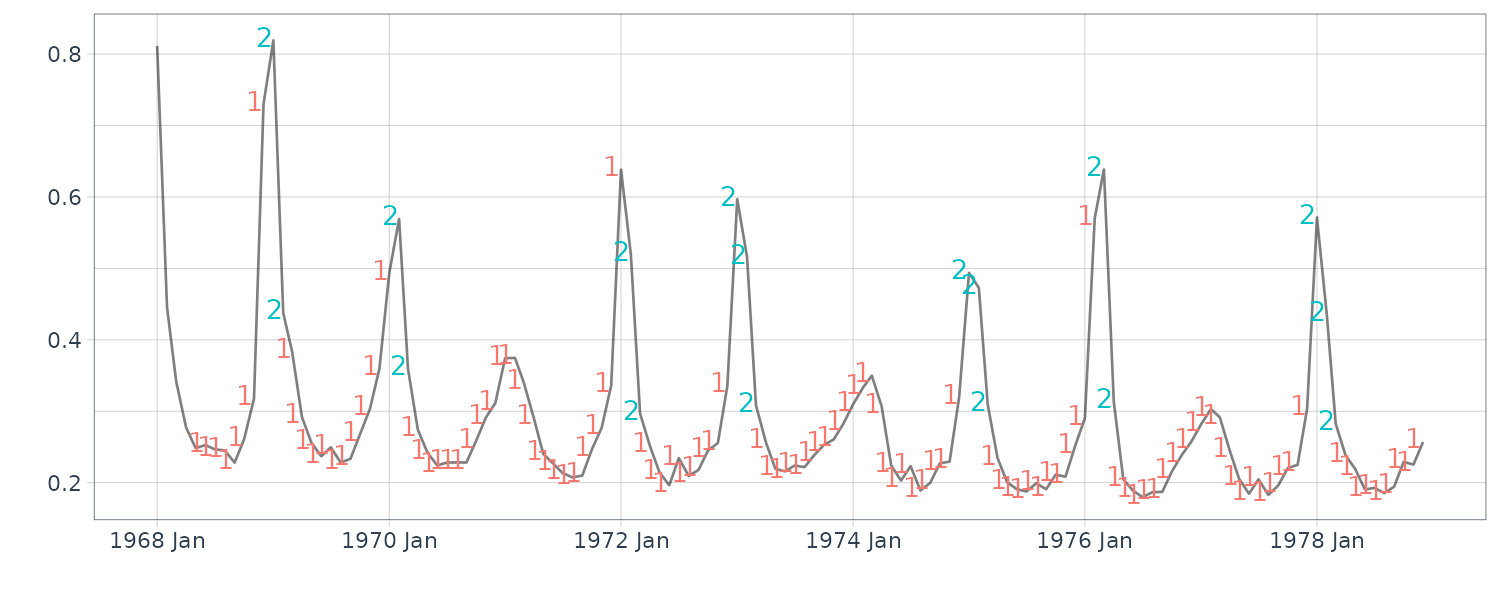   

And graphing \(x_{t1}, x_{t2}, x_{t3}\):

dat2 <- gather(dat, xt, value, xt1, xt2, xt3)

dat2 |>
  ggplot(aes(x = index, y = value, col = xt)) +    
  geom_line() +
  xlab("") +
  ylab("") +
  theme_tq()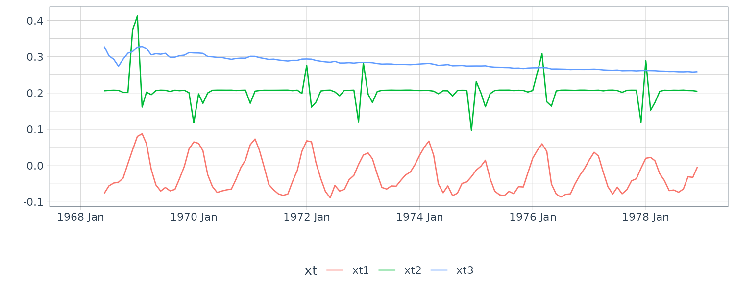

And with confidence intervals:

prde1 <- 2 * sqrt(innov.sig[1])
prde2 <- 2 * sqrt(innov.sig[2])
prde <- ifelse(predepi[k] < .5, prde1, prde2)    

dat <- dat |>
  mutate(
    prde = c(
      rep(NA, 5),
      ifelse(predepi[k] < .5, prde1, prde2)),
    yp = yp
  )

dat |>
  ggplot(aes(x = index, y = value)) +
  geom_ribbon(
    aes(
      ymax = yp + prde,
      ymin = yp - prde
    ),
    fill = "gray",
    alpha = 0.5
  ) +
  geom_point() +
  xlab("") +
  ylab("") +
  theme_tq()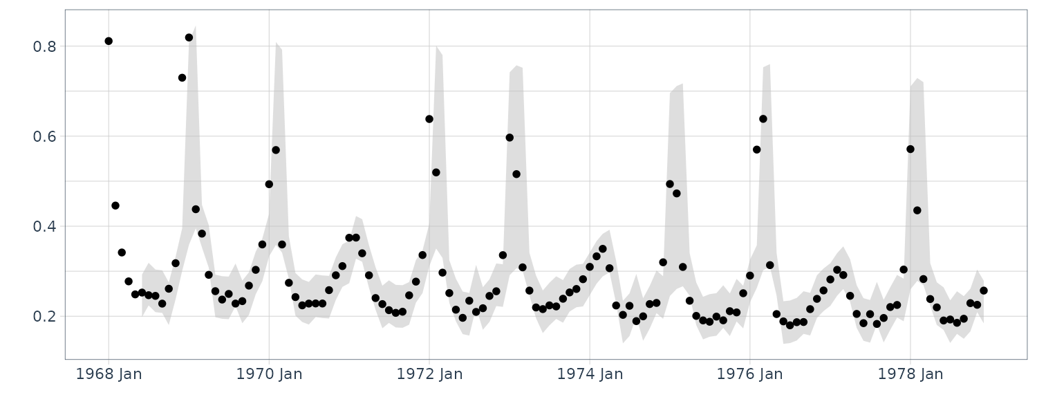

Bayesian Analysis of State Space Models

We now consider some Bayesian approaches to fitting linear Gaussian state space models via Markov chain Monte Carlo (MCMC) methods.

MCMC methods refer to Monte Carlo integration methods that use a Markovian updating scheme to sample from intractable posterior distributions. The most com- mon MCMC method is the Gibbs sampler, which is essentially a modification of the Metropolis algorithm. The basic strategy is to use conditional distributions to set up a Markov chain to obtain samples from a joint distribution.

Example: Gibbs Sampling for the Bivariate Normal

Suppose we wish to obtain samples from a bivariate normal distribution:

\[\begin{aligned} \begin{bmatrix} X\\ Y \end{bmatrix} &\sim N\Big( \begin{bmatrix} 0\\ 0 \end{bmatrix}, \begin{bmatrix} 1 & \rho\\ \rho & 1 \end{bmatrix} \Big) \end{aligned}\] \[\begin{aligned} |\rho| < 1 \end{aligned}\]

The problem is we can only generate samples from a univariate normal.

The univariate conditionals are:

\[\begin{aligned} (X|Y = y) &\sim N(\rho y, 1 - \rho^{2})\\ (Y|X = x) &\sim N(\rho x, 1 - \rho^{2})\\ \end{aligned}\]

And we can simulate from these distributions.

Construct a Markov chain. First Pick \(X^{(0)} = x_{0}\), and then iterate the process:

\[\begin{aligned} X^{(0)} = x_{0} &\rightarrow Y^{(0)}\\ \rightarrow X^{(1)} &\rightarrow Y^{(1)}\\ &\vdots\\ \rightarrow X^{(k)} &\rightarrow Y^{(k)}\\ &\vdots \end{aligned}\]

Where:

\[\begin{aligned} (Y^{(k)}|X^{(k)}= x_{k})\sim N(\rho x_{k}, 1 - \rho^{2})\\ (X^{(k)}|Y^{(k-1)}= y_{k-1})\sim N(\rho y_{k-1}, 1 - \rho^{2})\\ \end{aligned}\]

The joint distribution of \((X^{(k)}, Y^{(k)})\) is:

\[\begin{aligned} \begin{bmatrix} X^{(k)}\\ Y^{(k)} \end{bmatrix} &\sim N\Big( \begin{bmatrix} \rho^{2k}x_{0}\\ \rho^{2k+1}x_{0} \end{bmatrix}, \begin{bmatrix} 1 - \rho^{4k} & \rho(1 - \rho^{4k})\\ \rho(1 - \rho^{4k}) & 1 - \rho^{4k + 2} \end{bmatrix} \Big) \end{aligned}\]

Thus, for any starting value, \(x_{0}\):

\[\begin{aligned} \lim_{k \rightarrow \infty}(X^{(k)}, Y^{(k)}) \underset{d}{\rightarrow}(X, Y) \end{aligned}\]

The speed of convergence depends on ρ. Then one would run the chain and throw away the initial \(n_{0}\) sampled values (burnin) and retain the rest.

For state space models, the main objective is to obtain the posterior density of the parameters \(P(\boldsymbol{\Theta} \mid y_{1:n})\) or \(P(x_{0:n}\mid y_{1:n})\) if the states are meaningful. It is generally easier to get samples from the full posterior \(p(\boldsymbol{\Theta}, x_{0:n} \mid y_{1:n})\) and then marginalize (“average”) to obtain \(P(\boldsymbol{\Theta} \mid y_{1:n})\) or \(P(x_{0:n} \mid y_{1:n})\).

As previously mentioned, the most popular method is to run a full Gibbs sampler, alternating between sampling model parameters and latent state sequences from their respective full conditional distributions.

Gibbs Sampler Procedure for State Space Models:

Example: Local Level Model

Consider the model:

\[\begin{aligned} y_{t} &= x_{t} + v_{t}\\ x_{t} &= x_{t-1} + w_{t} \end{aligned}\] \[\begin{aligned} v_{t} &\sim N(0, \sigma_{v}^{2} = 1)\\ w_{t} &\sim N(0, \sigma_{w}^{2} = 0.5)\\ \end{aligned}\]

For the prior distributions, all parameters \((a_{0}, b_{0}, c_{0}, d_{0})\) were set to .02. We generated 1010 samples, using the first 10 as burn-in. The plot displays the simulated data and states, the contours of the likelihood of the data, the sampled posterior values as points, and the marginal sampled posteriors of each variance component along with the posterior means.

See Also

References

Shuway H. (2017) Time Series Analysis and Its Applications: With R Examples (Springer Texts in Statistics) 4th ed.