Econometrics (Time-Series Analysis)
Read PostIn this post, we will cover Carter R., Griffiths W., Lim G. (2018) Principles of Econometrics, focusing on time series analysis.
Contents:
- Introduction
- Modeling Dynamic Relationships
- Autocorrelation
- Stationarity
- Forecasting
- Granger Causality
- Testing for Serially Correlated Errors
- Time-Series Regressions for Policy Analysis
- Nonstationarity
- Unit Root Tests
- Cointegration
- Regression With No Cointegration
- Vector Autoregressive Models
- ARCH Models
- GARCH Models
- See Also
- References
Introduction
It is important to distinguish cross-sectional data and time-series data. Cross-sectional observations are typically collected by way of a random sample, and so they are uncorrelated. However, time-series observations, observed over a number of time periods, are likely to be correlated.
A second distinguishing feature of time-series data is a natural ordering to time. There is no such ordering in cross-sectional data and one could shuffle the observations. Time-series data often exhibit a dynamic relationship, in which the change in a variable now has an impact on the same or other variables in future time periods.
For example, it is common for a change in the level of an explanatory variable to have behavioral implications for other variables beyond the time period in which it occurred. The consequences of economic decisions that result in changes in economic variables can last a long time. When the income tax rate is increased, consumers have less disposable income, reducing their expenditures on goods and services, which reduces profits of suppliers, which reduces the demand for productive inputs, which reduces the profits of the input suppliers, and so on. The effect of the tax increase ripples through the economy. These effects do not occur instantaneously but are spread, or distributed, over future time periods.
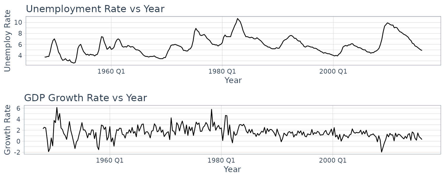
Example: Plotting the Unemployment Rate and the GDP Growth Rate for the United States
Using the dataset usmacro which contain the US quarterly unemployment rate and the US quarterly growth rate for GDP. We wish to understand how series such as these evolve over time, how current values of each data series are correlated with their past values, and how one series might be related to current and past values of another.
Plotting the unemployment rate and gdp growth rate:
usmacro$date <- as.Date(
  usmacro$dateid01,
  format = "%m/%d/%Y") |>
  yearquarter()

usmacro <- as_tsibble(
  usmacro,
  index = date
)

plot_grid(
  usmacro |>
    autoplot(u) +
    ylab("Unemployment Rate") +
    xlab("Year") +
    theme_tq(),
  usmacro |>
    autoplot(g) +
    ylab("Growth Rate") +
    xlab("Year") +
    theme_tq(),
  ncol = 1
)
Modeling Dynamic Relationships
Time-series data are usually dynamic. What this mean is their current values are correlated to their past values and current and past values of other variables. This particular dynamic relation can be modelled using lagged values such as:
\[\begin{aligned} y_{t-1}, y_{t-2}, \cdots, y_{t-q}\\ x_{t-1}, x_{t-2}, \cdots, x_{t-p}\\ e_{t-1}, e_{t-2}, \cdots, e_{t-s}\\ \end{aligned}\]In this section, we will describe a number of the time-series models that arise from introducing lags of these kinds and explore the relationships between them.
Finite Distributed Lag Models (FDL)
Suppose that \(y\) depends on current and lag value of \(x\):
\[\begin{aligned} y_{t} &= \alpha + \beta_{0}x_{t} + \beta_{1}x_{t - 1} + \cdots + + \beta_{q}x_{t-q} + e_{t} \end{aligned}\]It is called finite distributed lag because \(x\) cuts off after q lags and the impact of change in \(x\) is distributed over future time periods.
Model of this kind can be used for forecasting or policy analysis.
For example in forecasting, we might be interested in using information on past interest rates to forecast future inflation. And in policy analysis, a central bank might be interested in how inflation will react now and in the future to a change in the current interest rate.
Autoregressive Models (AR)
An autoregressive model is where \(y\) depends on past values of itself. An AR(p) model:
\[\begin{aligned} y_{t} &= \delta + \theta_{1}y_{t-1} + \cdots + \theta_{p}y_{t-p} + e_{t} \end{aligned}\]For example, an AR(2) model for the unemployment series would be:
\[\begin{aligned} U_{t} &= \delta + \theta_{1}U_{t-1} + \theta_{2}U_{t-2} + e_{t} \end{aligned}\]AR models can be used to describe time paths of variables and they are generally use for forecasting.
Autoregressive Distributed Lag Models (ARDL)
A more general case which includes autoregressive model and FDL model is the ARDL(p, q) model:
\[\begin{aligned} y_{t} &= \delta + \theta_{1}y_{t-1} + \cdots + \theta_{p}y_{t-p} + \beta_{0}x_{t} + \cdots \beta_{q}x_{t-q} + e_{t} \end{aligned}\]For example, an ARDL(2, 1) model relating the uemployment rate \(U\) to the economy \(G\):
\[\begin{aligned} U_{t} &= \delta + \theta_{1}U_{t-1} + \theta_{2}U_{t-2} + \beta_{0}G_{t} + \beta_{1}G_{t-1} + e_{t} \end{aligned}\]ARDL models can be used for both forecasting and policy analysis.
Infinite Distributed Lag Models (IDL)
An IDL Model is the same as FDL Model except it goes to infinity.
\[\begin{aligned} y_{t} &= \alpha + \beta_{0}x_{t} + \beta_{1}x_{t-1} + \cdots \beta_{q}x_{t-q} + \cdots + e_{t} \end{aligned}\]In order to make the model realistic, \(\beta_{s}\) has to eventually decline to 0.
There are many possible lag pattern, but a popular one is the geometrically declining lag pattern:
\[\begin{aligned} \beta_{s} &= \lambda^{s}\beta_{0} \end{aligned}\] \[\begin{aligned} y_{t} &= \alpha + \beta_{0}x_{t} + \lambda\beta_{0}x_{t-1} + \lambda^{2}\beta_{0}x_{t-2} + \cdots + e_{t} \end{aligned}\] \[\begin{aligned} 0 < \lambda < 1 \end{aligned}\]It is possible to change an geometrically decaying IDL into an ARDL(1, 0):
\[\begin{aligned} y_{t} &= \alpha + \beta_{0}x_{t} + \lambda\beta_{0}x_{t-1} + \lambda^{2}\beta_{0}x_{t-2} + \cdots + e_{t}\\[5pt] y_{t-1} &= \alpha + \beta_{0}x_{t-1} + \lambda\beta_{0}x_{t-2} + \lambda^{2}\beta_{0}x_{t-3} + \cdots + e_{t}\\[5pt] \lambda y_{t-1} &= \lambda\alpha + \lambda\beta_{0}x_{t-1} + \lambda^{2}\beta_{0}x_{t-2} + \lambda^{3}\beta_{0}x_{t-3} + \cdots + \lambda e_{t} \end{aligned}\] \[\begin{aligned} y_{t} - \lambda y_{t-1} &= \alpha(1 - \lambda) + \beta_{0}x_{t} + e_{t} - \lambda e_{t-1} \end{aligned}\] \[\begin{aligned} y_{t} &= \alpha(1 - \lambda) + \lambda y_{t-1} + \beta_{0}x_{t} + e_{t} - \lambda e_{t-1}\\ y_{t} &= \delta + \theta y_{t-1} + \beta_{0}x_{t} + v_{t} \end{aligned}\] \[\begin{aligned} \delta &= \alpha(1 - \lambda)\\ \theta &= \lambda\\ v_{t} &= e_{t} - \lambda e_{t-1} \end{aligned}\]It is also possible to turn an ARDL model into an IDL model. Generally, ARDL(p, q) models can be transformed into IDL models as long as the lagged coefficients eventually decline to 0.
The ARDL formulation is useful for forecasting while the IDL provides useful information for policy analysis.
Autoregressive Error Models
Another way in which lags can enter a model is through the error term:
\[\begin{aligned} e_{t} &= \rho e_{t-1} + v \end{aligned}\]In contrast to AR model, there is no intercept parameter as \(e_{t}\) has a zero mean.
Let’s include this error term in a model:
\[\begin{aligned} y_{t} &= \alpha + \beta_{0}x_{t} + e_{t}\\ &= \alpha + \beta_{0}x_{t} + \rho e_{t-1} + v_{t}\\ \end{aligned}\]\(e_{t-1}\) can be written as:
\[\begin{aligned} y_{t-1} &= \alpha + \beta_{0}x_{t-1} + e_{t-1}\\ e_{t-1} &= y_{t-1} - \alpha - \beta_{0}x_{t-1}\\ \rho e_{t-1} &= \rho y_{t-1} - \rho \alpha - \rho \beta_{0}x_{t-1} \end{aligned}\]We can then turn a AR(1) error model into an ARDL(1, 1) model:
\[\begin{aligned} y_{t} &= \alpha + \beta_{0}x_{t} + \rho e_{t-1} + v\\ &= \alpha + \beta_{0}x_{t} + (\rho y_{t-1} - \rho \alpha - \rho \beta_{0}x_{t-1}) + v\\ &= \alpha(1 - \rho) + \rho y_{t-1} + \beta_{0}x_{t} - \rho \beta_{0}x_{t-1} + v_{t}\\ &= \delta + \theta y_{t-1} + \beta_{0}x_{t} + \beta_{1}x_{t-1} + v_{t} \end{aligned}\] \[\begin{aligned} y_{t} &= \delta + \theta y_{t-1} + \beta_{0}x_{t} + \beta_{1}x_{t-1} + v_{t} \end{aligned}\] \[\begin{aligned} \delta &= \alpha(1 - \rho)\\ \theta &= \rho \end{aligned}\]Note that we have a constraint here which is not in a general ARDL model and nonlinear:
\[\begin{aligned} \beta_{1} &= -\rho\beta_{0} \end{aligned}\]Autoregressive error models with more lags than one can also be transformed to special cases of ARDL models.
Summary of Dynamic Models for Stationary Time Series Data
ARDL(p, q) Model
\[\begin{aligned} y_{t} &= \delta + \theta_{1}y_{t-1} + \cdots + \theta_{p}y_{t-p} + \beta_{0}x_{t} + \cdots \beta_{q}x_{t-q} + e_{t} \end{aligned}\]FDL Model
\[\begin{aligned} y_{t} &= \alpha + \beta_{0}x_{t} + \beta_{1}x_{t - 1} + \cdots + \beta_{q}x_{t-q} + e_{t} \end{aligned}\]IDL Model
\[\begin{aligned} y_{t} &= \alpha + \beta_{0}x_{t} + \beta_{1}x_{t-1} + \cdots + e_{t} \end{aligned}\]AR(p) Model
\[\begin{aligned} y_{t} &= \delta + \theta_{1}y_{t-1} + \cdots + \theta_{p}y_{t-p} + e_{t} \end{aligned}\]IDL model with Geometrically Declining Lag Weights
\[\begin{aligned} \beta_{S} &= \lambda^{S}\beta_{0} \end{aligned}\] \[\begin{aligned} 0 < \lambda < 1 \end{aligned}\] \[\begin{aligned} y_{t} &= \alpha(1 - \lambda) + \lambda y_{t-1} + \beta_{0}x_{t} + e_{t} - \lambda e_{t-1} \end{aligned}\]Simple Regression with AR(1) Error
\[\begin{aligned} y_{t} &= \alpha + \beta_{0}x_{t} + e_{t}\\ e_{t} &= \rho e_{t-1} + v_{t} \end{aligned}\] \[\begin{aligned} y_{t} &= \alpha(1 - \rho) + \rho y_{t-1} + \beta_{0}x_{t} - \rho \beta_{0}x_{t-1} + v_{t} \end{aligned}\]How we interpret each model depends on whether the model is used for forecasting or policy analysis. On assumption we make for all models is that the variables in the models are stationary and weakly dependent.
Autocorrelation
Consider a time series of observations, \(x_{1}, \cdots, x_{T}\) with:
\[\begin{aligned} E[x_{t}] &= \mu_{X}\\ \text{var}(x_{t}) &= \sigma_{X}^{2} \end{aligned}\]We assume the mean and variance do not change over time. The population autocorrleation that are s periods apart:
\[\begin{aligned} \rho_{s} &= \frac{\mathrm{Cov}(x_{t}, x_{t-s})}{\mathrm{Var(x_{t})}} \end{aligned}\] \[\begin{aligned} x &= 1, 2, \cdots \end{aligned}\]Sample Correlation
Population autocorrelations theoretically require a conceptual time series that goes on forever, from the infinite past and continuing to the infinite future. Sample autocorrelations are a sample of observations for a finite time period to estimate the population autocorrelations.
To estimate \(\rho_{1}\):
\[\begin{aligned} \hat{\text{cov}}(x_{t}, x_{t-1}) &= \frac{1}{T}\sum_{t=2}^{T}(x_{t} - \bar{x})(x_{t-1} - \bar{x})\\ \hat{\text{var}}(x_{t}) &= \frac{1}{T-1}\sum_{t=1}^{T}(x_{t} - \bar{x})^{2} \end{aligned}\] \[\begin{aligned} r_{1} &= \frac{\sum_{t=2}^{T}(x_{t}- \bar{x})(x_{t-1} - \bar{x})}{\sum_{t=1}^{T}(x_{t}-\bar{x})^{2}} \end{aligned}\]More generally:
\[\begin{aligned} r_{s} &= \frac{\sum_{t=s+1}^{T}(x_{t} - \bar{x})(x_{t-s} - \bar{x})}{\sum_{t=1}^{T}(x_{t} - \bar{x})^{2}} \end{aligned}\]Because only \((T-s)\) observations are used to compute the numerator and \(T\) observations are used to compute the denominator, an alternative calculation that leads to a larger estimate is:
\[\begin{aligned} r'_{s} &= \frac{\frac{1}{T-s}\sum_{t=s+1}^{T}(x_{t} - \bar{x})(x_{t-s} - \bar{x})}{\frac{1}{T}\sum_{t=1}^{T}(x_{t} - \bar{x})^{2}} \end{aligned}\]Test of Significance
Assuming the null hypothesis as \(H_{0}: \rho_{s} = 0\) is true, \(r_{s}\) has an approximate normal distribution:
\[\begin{aligned} r_{s} \sim N\Big(0, \frac{1}{T}\Big) \end{aligned}\]Standardizing \(\hat{\rho}_{s}\):
\[\begin{aligned} Z &= \frac{r_{s} - 0}{\sqrt{\frac{1}{T}}}\\[5pt] &= \sqrt{T}r_{s}\\[5pt] Z &\sim N(0, 1) \end{aligned}\]Correlogram
Also called the sample ACF, the correlogram is the sequence of autocorrelations \(r_{1}, r_{2}, \cdots\).
We say that \(r_{s}\) is significantly different from 0 at a 5% significance if:
\[\begin{aligned} \sqrt{T}r_{s} &\leq -1.96\\ \sqrt{T}r_{s} &\geq 1.96 \end{aligned}\]Example: Sample Autocorrelations for Unemployment
Consider the quarterly series for the U.S. unemployment rate found in the dataset usmacro.
The horizontal line is drawn at:
\[\begin{aligned} \pm\frac{1.96}{\sqrt{T}} &= \frac{1.96}{\sqrt{173}}\\[5pt] &= \pm 0.121 \end{aligned}\]usmacro |>
ACF(u) |>
autoplot() +
ggtitle("ACF") +
theme_tq()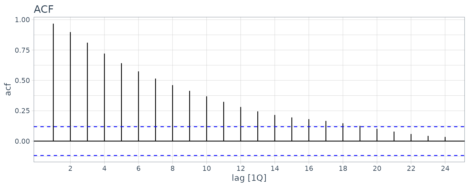
Example: Sample Autocorrelations for GDP Growth Rate
The autocorrelations are smaller than those for the unemployment series, but there’s a series of pattern where the correlations oscillate between signifcance and insignificance. This could be due to the business cycle.
usmacro |>
  ACF(g, lag_max = 48) |>
  autoplot() +
  scale_x_continuous(
    breaks = seq(0, 48, 5)
  )+
  ggtitle("ACF") +
  theme_tq()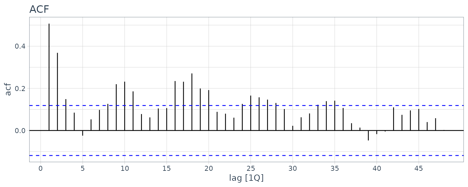
Stationarity
Stationarity means the mean and variances do not change over time and autocorrelation between variables depend only on how far apart they are in time. Another way to think of this is if you take any subset of the time series, they will have the same mean, variance, and \(\rho{1}, \rho_{2}, \cdots\). Up till now, we have assumed in the modeling that the variables are stationary.
Test of stationarity with “Unit Root Test” can be taken to detect non-stationarity which will cover later.
In addition to assuming that the variables are stationary, we also assume they are weakly dependent. Weak dependence implies that as \(s \rightarrow \infty\), \(x_{t}, x_{t+s}\) are becoming independent. In other words, as s grows larger, the autocorrelation decreases to zero. Stationary variables typically have weak dependence but not always.
Stationary variables need to be weakly dependent in order for the least squares estimator to be consistent.
Example: Are the Unemployment and Growth Rate Series Stationary and Weakly Dependent?
We will answer the question of stationarity in terms of formal test later when we cover unit root test. For now, we graph the ACFs:
usmacro |>
  ACF(u) |>
  autoplot() +
  ggtitle("ACF (Unemployment Rate)") +
  theme_tq()

usmacro |>
  ACF(g) |>
  autoplot() +
  ggtitle("ACF (GDP Growth Rate)") +
  theme_tq()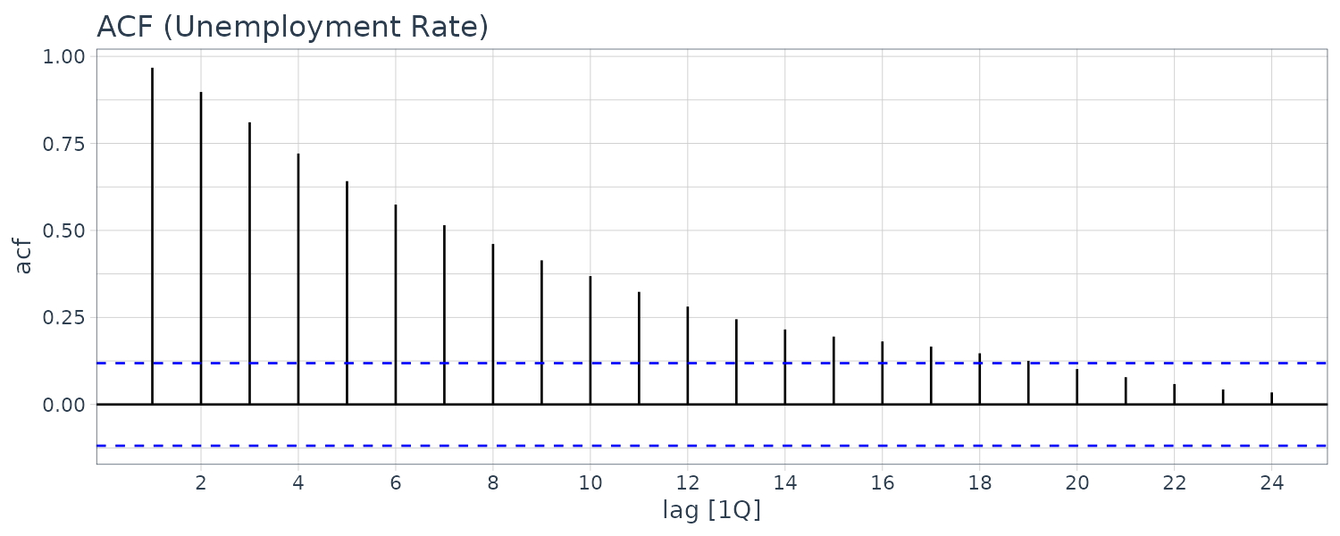
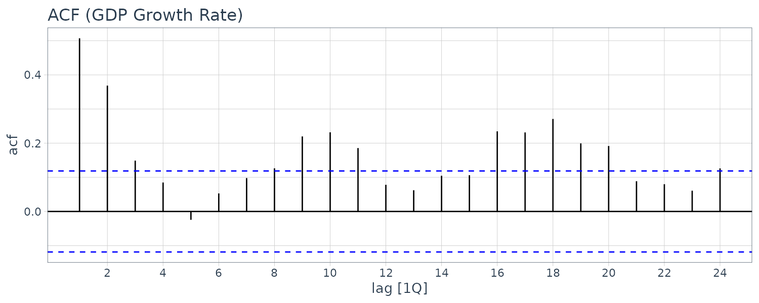
We can see that the autocorrelations die out pretty quickly so we conclude it is weakly dependent. But we cannot ascertain whether it is stationary from the correlogram. It turns out that unemployment rate is indeed stationary.
GDP growth rate looks more stationary and certainly weakly dependent.
Knowing the unemployment and growth rates are stationary and weakly dependent means that we can proceed to use them for time-series regression models with stationary variables. With the exception of a special case known as cointegration, variables in time-series regressions must be stationary and weakly dependent for the least squares estimator to be consistent.
Forecasting
In this section, we consider forecasting using two different models, an AR model, and an ARDL model. The focus is on short-term forecasting, typically up to three periods into the future.
Suppose we have the following ARDL(2, 2) model:
\[\begin{aligned} y_{t} &= \delta + \theta_{1}y_{t-1} + \theta_{2}y_{t-2} + \beta_{1}x_{t-1} + \beta_{2}x_{t-2} + e_{t} \end{aligned}\]Notice that the term \(x_{t}\) is missing. The reason is it is unlikely that \(x_{t}\) will be observed at the time of forecast so the omission is desirable.
Hence the ARDL forecast equation would be:
\[\begin{aligned} y_{T+1} &= \delta + \theta_{1}y_{T} + \theta_{2}y_{T-1} + \beta_{1}x_{T} + \beta_{2}x_{T-1} + e_{t} \end{aligned}\]Defining the information set to be the set of all current and past observations of \(y\) and \(x\) at time \(t\) as:
\[\begin{aligned} I_{t} &= {y_{t}, y_{t-1}, \cdots, x_{t}, x_{t-1}, \cdots} \end{aligned}\]Assuming that we are standing at the end of the sample period, having observed \(y_{T}, x_{T}\), the one-period ahead forecasting problem is to find a forecast \(\hat{y}_{T+1}\mid I_{T}\).
The best forecast in a minimizing the conditional mean-squared forecast error :
\[\begin{aligned} E[(\hat{y}_{T+1} - y_{T+1})^{2}\mid I_{T}] \end{aligned}\]Is the conditional expectation:
\[\begin{aligned} \hat{y}_{T+1} &= E[Y_{T+1}\mid I_{t}] \end{aligned}\]For example, suppose we believe only 2 lags of \(y, x\) are relevant, we are assuming that:
\[\begin{aligned} E[y_{T+1}\mid I_{t}] &= E[y_{T+1}\mid y_{T}, y_{T - 1}, x_{T}, x_{T-1}]\\ &= \delta + \theta_{1}y_{T-1} + \theta_{2}y_{T-2} + \beta_{1}x_{T-1} + \beta_{2}x_{T-2} \end{aligned}\]By employing an ARDL(2, 2) model, we are assuming that, for forecasting \(y_{T+1}\) , observations from more than two periods in the past do not convey any extra information relative to that contained in the most recent two observations.
Furthermore, we require:
\[\begin{aligned} E[e_{T+1}\mid I_{T}] &= 0 \end{aligned}\]For 2-period and 3-period ahead forecasts:
\[\begin{aligned} \hat{y}_{T + 2} = \ &E[y_{T+2}\mid I_{T}]\\[5pt] = \ &\delta + \theta E[Y_{T+1}\mid I_{T}] + \theta_{2}y_{T}\ + \\ &\beta_{1}E[x_{T+1}\mid I_{t}] + \beta_{2}x_{T} \end{aligned}\] \[\begin{aligned} \hat{y}_{T + 3} = \ &E[y_{T+3}\mid I_{T}]\\[5pt] = \ &\delta + \theta E[Y_{T+2}\mid I_{T}] + \theta_{2}E[Y_{T+1}\mid I_{T}]\ + \\ &\beta_{1}E[x_{T+2}\mid I_{t}] + \beta_{2}E[X_{T + 1}\mid I_{T}] \end{aligned}\]Note that we have estimate of \(E[y_{T+2} \mid I_{T}], [y_{T+1} \mid I_{T}]\) from previous period’s forecasts, but \([x_{T+2} \mid I_{T}], [x_{T+1} \mid I_{T}]\) require extra information. They could be derived from independent forecasts or in what-if type scenarios. If the model is a pure AR model, this issue does not arise.
Example: Forecasting Unemployment with an AR(2) Model
To demonstrate how to use an AR model for forecasting, we consider this AR(2) model for forecasting US unemployment rate:
\[\begin{aligned} U_{t} &= \delta + \theta_{1}U_{t-1} + \theta_{2}U_{t-2} + e_{t} \end{aligned}\]We assume that past values of unemployment cannot be used to forecast the error in the current period:
\[\begin{aligned} E[e_{t} \mid I_{t-1}] &= 0 \end{aligned}\]The expressions for forecasts for the remainder of 2016:
\[\begin{aligned} \hat{U}_{2016Q2} &= E[U_{2016Q2}\mid I_{2016Q1}]\\[5pt] &= \delta + \theta_{1}U_{2016Q1} + \theta_{2}U_{2015Q4} \end{aligned}\] \[\begin{aligned} \hat{U}_{2016Q3} &= E[U_{2016Q3}\mid I_{2016Q1}]\\[5pt] &= \delta + \theta_{1}E[U_{2016Q2}\mid I_{2016Q1}] + \theta_{2}U_{2016Q1} \end{aligned}\] \[\begin{aligned} \hat{U}_{2016Q4} &= E[U_{2016Q4}\mid I_{2016Q1}]\\[5pt] &= \delta + \theta_{1}E[U_{2016Q3}\mid I_{2016Q1}] + \theta_{2}E[U_{2016Q2}\mid I_{2016Q_{1}}] \end{aligned}\]Example: OLS Estimation of the AR(2) Model for Unemployment
The assumption that \(E[e_{t}\mid I_{t-1}] = 0\) is sufficient for the OLS estimator to be consistent. However, the OLS estimator will be biased, but consistency gives it a large-sample justification. The reason it is biased is because even though:
\[\begin{aligned} \text{cov}(e_{t}, y_{t-s}) &= 0\\ \text{cov}(e_{t}, x_{t-s}) &= 0 \end{aligned}\] \[\begin{aligned} s &> 0 \end{aligned}\]It does not mean future values will not be correlated with \(e_{t}\), which is a condition for the estimator to be unbiased. In other words, the assumption of \(E[e_{t}\mid I_{t-1}]\) is weaker than the strict exogeneity assumption.
The OLS estimates yields the following equation:
\[\begin{aligned} \hat{U}_{t} &= 0.2885 + 1.6128 U_{t-1} - 0.6621 U_{t-2} \end{aligned}\] \[\begin{aligned} \hat{\sigma} &= 0.2947 \end{aligned}\] \[\begin{aligned} \text{se}(\theta_{0}) &= 0.0666\\ \text{se}(\theta_{1}) &= 0.0457\\ \text{se}(\theta_{2}) &= 0.0456 \end{aligned}\]The standard error and \(\hat{\sigma}\) estimates will be valid if the conditional homoskedasticity assumption is true:
\[\begin{aligned} \text{var}(e_{t}\mid U_{t-1}, U_{t-2}) &= \sigma^{2} \end{aligned}\]We can show this in R:
fit <- usmacro |>
  model(
    ARIMA(
      u ~ 1 +
        lag(u, 1) +
        lag(u, 2) +
        pdq(0, 0, 0) +
        PDQ(0, 0, 0)
    )
  )

> tidy(fit) |>
  select(-.model)
# A tibble: 3 × 5
  term      estimate std.error statistic   p.value
  <chr>        <dbl>     <dbl>     <dbl>     <dbl>
1 lag(u, 1)    1.61     0.0454     35.5  6.95e-104
2 lag(u, 2)   -0.662    0.0453    -14.6  4.80e- 36
3 intercept    0.289    0.0662      4.36 1.88e-  5

> report(fit)
Series: u
Model: LM w/ ARIMA(0,0,0) errors

Coefficients:
      lag(u, 1)  lag(u, 2)  intercept
         1.6128    -0.6621     0.2885
s.e.     0.0454     0.0453     0.0662

sigma^2 estimated as 0.08621:  log likelihood=-51.92
AIC=111.84   AICc=111.99   BIC=126.27
Example: Unemployment Forecasts
Having now the OLS estimates, we can use it for forecasting:
\[\begin{aligned} \hat{U}_{2016Q2} &= \hat{\delta} + \hat{\theta_{1}}U_{2016Q1} + \hat{\theta_{2}}U_{2015Q4}\\ &= 0.28852 + 1.61282 \times 4.9 - 0.66209 \times 5\\ &= 4.8809 \end{aligned}\] \[\begin{aligned} U_{2016Q1} &= 4.9\\ U_{2015Q4} &= 5 \end{aligned}\]Two quarters ahead forecast:
\[\begin{aligned} \hat{U}_{2016Q3} &= \hat{\delta} + \hat{\theta_{1}}\hat{U}_{2016Q2} + \hat{\theta_{2}}U_{2016Q1}\\ &= 0.28852 + 1.61282 \times 4.8809 - 0.66209 \times 4.9\\ &= 4.9163 \end{aligned}\] \[\begin{aligned} \hat{U}_{2016Q2} &= 4.8809\\ U_{2016Q1} &= 4.9 \end{aligned}\]Two quarters ahead forecast:
\[\begin{aligned} \hat{U}_{2016Q4} &= \hat{\delta} + \hat{\theta_{1}}\hat{U}_{2016Q3} + \hat{\theta_{2}}\hat{U}_{2016Q2}\\ &= 0.28852 + 1.61282 \times 4.9163 - 0.66209 \times 4.8809\\ &= 4.986 \end{aligned}\] \[\begin{aligned} \hat{U}_{2016Q3} &= 4.9163\\ \hat{U}_{2016Q2} &= 4.8809 \end{aligned}\]Forecast Intervals and Standard Errors
Given the general ARDL(2, 2) model:
\[\begin{aligned} y_{t} &= \delta + \theta_{1}y_{t-1} + \theta_{2}y_{t-2} + \beta_{1}x_{t-1} + \beta_{2}x_{t-2} + e_{t} \end{aligned}\]The one-period ahead forecast error \(f_{1}\) is given by:
\[\begin{aligned} f_{1} &= y_{T+1} - \hat{y}_{T+1}\\ &= (\delta - \hat{\delta}) + (\theta_{1}- \hat{\theta}_{1})y_{T} + (\theta_{2} - \hat{\theta}_{2})y_{T-2} + (\beta_{1}- \hat{\beta}_{1})x_{T-1} + (\beta_{2} - \hat{\beta}_{2})x_{T-2} + e_{T+1} \end{aligned}\]To simplify calculation, we ignore the error from estimating the coefficients. The coefficients error in most cases pales with comparison with the variance of the random error. Using this simplication we have:
\[\begin{aligned} f_{1} &= e_{T+1} \end{aligned}\]For two-periods ahead forecast:
\[\begin{aligned} \hat{y}_{T+2} &= \delta + \theta_{1}\hat{y}_{T+1} + \theta_{2}y_{T} + \beta_{1}\hat{x}_{T+1} + \beta_{2}x_{T} \end{aligned}\]Assuming that the values for \(\hat{x}_{T+1}\) are given in a what-if scenario:
\[\begin{aligned} \hat{y}_{T+2} &= \delta + \theta_{1}\hat{y}_{T+1} + \theta_{2}y_{T} + \beta_{1}x_{T+1} + \beta_{2}x_{T} \end{aligned}\]And the actual two-period ahead:
\[\begin{aligned} y_{T+2} &= \delta + \theta_{1} y_{T+1} + \theta_{2}y_{T} + \beta_{1}x_{T+1} + \beta_{2}x_{T} + e_{T+2} \end{aligned}\]Then the two-period ahead forecast error is:
\[\begin{aligned} f_{2} &= y_{T+2} - \hat{y}_{T+2}\\ &= \theta_{1}(y_{T+1} - \hat{y}_{T+1}) + e_{T+2}\\ &= \theta_{1} f_{1} + e_{T+2}\\ &= \theta_{1}e_{T+1} + e_{T+2} \end{aligned}\]For the estimated three-period ahead and assuming that the values for \(\hat{x}_{T+1}\) are given in a what-if scenario:
\[\begin{aligned} \hat{y}_{T+3} &= \delta + \theta_{1}\hat{y}_{T+2} + \theta_{2}\hat{y}_{T+1} + \beta_{1}x_{T+2} + \beta_{2}x_{T+1} \end{aligned}\]And the actual three-period ahead:
\[\begin{aligned} y_{T+3} &= \delta + \theta_{1} y_{T+2} + \theta_{2}\hat{y}_{T+1} + \beta_{1}x_{T+2} + \beta_{2}x_{T+1} + e_{T+3} \end{aligned}\]Then the three-period ahead forecast error is:
\[\begin{aligned} f_{3} &= y_{T+3} - \hat{y}_{T+3}\\ &= \theta_{1}(y_{T+2} - \hat{y}_{T+2}) + \theta_{2}(y_{T+1} - \hat{y}_{T+1}) + e_{T+3}\\ &= \theta_{1} f_{2} + \theta_{2}f_{1} + e_{T+3}\\ &= \theta_{1}(\theta_{1}e_{T+1} + e_{T+2}) + \theta_{2}(e_{T+1}) + e_{T+3}\\ &= \theta_{1}^{2}e_{T+1} + \theta_{1}e_{T+2} + \theta_{2}e_{T+1} + e_{T+3}\\ &= (\theta_{1}^{2} + \theta_{2})e_{T+1} + \theta_{1}e_{T+2} + e_{T+3} \end{aligned}\]For the estimated 4-period ahead:
\[\begin{aligned} \hat{y}_{T+4} &= \delta + \theta_{1}\hat{y}_{T+3} + \theta_{2}\hat{y}_{T+2} + \beta_{1}x_{T+3} + \beta_{2}x_{T+2} \end{aligned}\]And the actual 4-period ahead:
\[\begin{aligned} y_{T+4} &= \delta + \theta_{1} y_{T+3} + \theta_{2}\hat{y}_{T+2} + \beta_{1}x_{T+3} + \beta_{2}x_{T+2} + e_{T+4} \end{aligned}\]Then the 4-period ahead forecast error is:
\[\begin{aligned} f_{4} &= y_{T+4} - \hat{y}_{T+4}\\ &= \theta_{1}(y_{T+3} - \hat{y}_{T+3}) + \theta_{2}(y_{T+2} - \hat{y}_{T+2}) + e_{T+4}\\ &= \theta_{1} f_{3} + \theta_{2}f_{2} + e_{T+4}\\ &= \theta_{1}((\theta_{1}^{2} + \theta_{2})e_{T+1} + \theta_{1}e_{T+2} + e_{T+3}) + \theta_{2}(\theta_{1}e_{T+1} + e_{T+2}) + e_{T+4}\\ &= \theta_{1}^{3}e_{T+1} + \theta_{2}\theta_{1}e_{T+1} + \theta_{1}^{2}e_{T+2} + \theta_{1}e_{T+3} + \theta_{2}\theta_{1}e_{T+1} + \theta_{2}e_{T+2} + e_{T+4}\\ &= (\theta_{1}^{3} + 2\theta_{2}\theta_{1} + \theta_{1}^{2})e_{T+1} + (\theta_{1}^{2} + \theta_{2})e_{T+2} + \theta_{1}e_{T+3}+ e_{T+4} \end{aligned}\]Taking variance of the error we get:
\[\begin{aligned} \sigma_{f1}^{2} &= \text{var}(f_{1}\mid I_{T})\\ &= \sigma^{2}\\[5pt] \sigma_{f2}^{2} &= \text{var}(f_{2}\mid I_{T})\\ &= \sigma^{2}(1 + \theta_{1}^{2})\\[5pt] \sigma_{f3}^{2} &= \text{var}(f_{3}\mid I_{T})\\ &= \sigma^{2}[(\theta_{1}^{2} + \theta_{2})^{2} + \theta_{1}^{2} + 1]\\ \sigma_{f4}^{2} &= \text{var}(f_{4}\mid I_{T})\\[5pt] &= \sigma^{2}[(\theta_{1}^{3} + 2\theta_{1}\theta_{2} + \theta_{2})^{2} + (\theta_{1}^{2} + \theta_{2})^{2} + \theta_{1}^{2} + 1]\\ \end{aligned}\]Example: Forecast Intervals for Unemployment from the AR(2) Model
Given the following AR(2) model:
\[\begin{aligned} U_{t} &= \delta + \theta_{1}U_{t-1} + \theta_{2}U_{t-2} + e_{t} \end{aligned}\]To forecast in R, we first fit the model using fable:
fit <- usmacro |>
  model(ARIMA(u ~ pdq(2, 0, 0) + PDQ(0, 0, 0)))

> tidy(fit) |>
  select(-.model)
# A tibble: 3 × 5
  term     estimate std.error statistic   p.value
  <chr>       <dbl>     <dbl>     <dbl>     <dbl>
1 ar1         1.61     0.0449      35.9 2.09e-105
2 ar2        -0.661    0.0451     -14.7 2.44e- 36
3 constant    0.278    0.0174      16.0 4.77e- 41
The coefficients are slightly different because fable uses MLE while the book uses OLS. As the forecast variance calculation is not directly supported:
fit <- usmacro |>
  model(
    ARIMA(
      u ~ 1 +
        lag(u, 1) +
        lag(u, 2) +
        pdq(0, 0, 0) +
        PDQ(0, 0, 0)
    )
  )

> tidy(fit) |>
  select(-.model)
# A tibble: 3 × 5
  term      estimate std.error statistic   p.value
  <chr>        <dbl>     <dbl>     <dbl>     <dbl>
1 lag(u, 1)    1.61     0.0454     35.5  6.95e-104
2 lag(u, 2)   -0.662    0.0453    -14.6  4.80e- 36
3 intercept    0.289    0.0662      4.36 1.88e-  5
To forecast in R:
fcast <- fit |>
  forecast(h = 3) |>
  hilo(95) |>
  select(-.model)

> fcast
# A tsibble: 3 x 4 [1Q]
     date             u .mean                  `95%`
    <qtr>        <dist> <dbl>                 <hilo>
1 2016 Q2 N(4.9, 0.087)  4.87 [4.297622, 5.452135]95
2 2016 Q3  N(4.9, 0.31)  4.90 [3.804995, 5.995970]95
3 2016 Q4    N(5, 0.64)  4.96 [3.391705, 6.525075]95
And the standard errors:
> sqrt(distributional::variance(fcast$u))
[1] 0.2945241 0.5589325 0.7993436
And graphing the forecast:
fit |>
  forecast(h = 3) |>
  autoplot(usmacro) +
  theme_tq()
Example: Forecasting Unemployment with an ARDL(2, 1) Model
We include a lagged value of the growth rate of the GDP. The OLS model is:
\[\begin{aligned} \hat{U}_{t} &= 0.3616 + 1.5331 U_{t-1} - 0.5818 U_{t-2} - 0.04824 G_{t-1} \end{aligned}\]Unfortunately fable doesn’t support ARDL models directly. However we can do this using the dLagM package:
library(dLagM)

usmacro$g1 <- lag(usmacro$g)

rem.p <- list(
  g1 = c(1)
)
rem.q <- c()

remove <- list(
  p = rem.p, q = rem.q
)

fit <- ardlDlm(
  u ~ g1,
  p = 1,
  q = 2,
  data = usmacro,
  remove = remove
)

> summary(fit)
Time series regression with "ts" data:
Start = 3, End = 273

Call:
dynlm(formula = as.formula(model.text), data = data)

Residuals:
     Min       1Q   Median       3Q      Max
-0.83591 -0.17311 -0.02963  0.15226  1.20016

Coefficients:
            Estimate Std. Error t value Pr(>|t|)
(Intercept)  0.36157    0.07228   5.002 1.03e-06 ***
g1.t        -0.04824    0.01949  -2.475   0.0139 *
u.1          1.53310    0.05555  27.597  < 2e-16 ***
u.2         -0.58179    0.05559 -10.465  < 2e-16 ***
---
Signif. codes:  0 ‘***’ 0.001 ‘**’ 0.01 ‘*’ 0.05 ‘.’ 0.1 ‘ ’ 1

Residual standard error: 0.2919 on 267 degrees of freedom
Multiple R-squared:  0.9685,	Adjusted R-squared:  0.9681
F-statistic:  2734 on 3 and 267 DF,  p-value: < 2.2e-16
We can see that the above result matches the OLS estimates.
Using a what-if scenario, we assume that:
\[\begin{aligned} G_{2016Q2} &= 0.869\\ G_{2016Q3} &= 1.069 \end{aligned}\]fcast <- dLagM::forecast(
fit,
x = c(0.31, 0.869, 1.069),
h = 3,
interval = TRUE
)
> fcast
$forecasts
95% LB Forecast 95% UB
1 4.402419 4.949870 5.522786
2 4.139368 5.057540 6.107228
3 3.842399 5.183947 6.747698
$call
forecast.ardlDlm(model = fit,
x = c(0.31, 0.869, 1.069),
h = 3, interval = TRUE)
attr(,"class")
[1] "forecast.ardlDlm" "dLagM" To retrieve the standard errors:
> (fcast$forecasts[, 3] - fcast$forecasts[, 2]) / 1.96
[1] 0.2923041 0.5355552 0.7978317
In fable, we can use the autocorrelation of the error to get similar coefficients. Note that the intercept is different from ARDL as the equation is fundamentally different. The coefficients are slightly different due to MLE vs OLS:
\[\begin{aligned} \hat{U}_{t} &= 5.76 - 0.00574 G_{t-1} + e_{t}\\ e_{t} &= 1.61 e_{t-1} - 0.659 e_{t-2} \end{aligned}\]fit <- usmacro |>
model(
ARIMA(
u ~ lag(g) +
pdq(2, 0, 0) +
PDQ(0, 0, 0)
)
)
> tidy(fit) |>
select(-.model)
# A tibble: 4 × 5
term estimate std.error statistic p.value
<chr> <dbl> <dbl> <dbl> <dbl>
1 ar1 1.61 0.0454 35.5 4.25e-104
2 ar2 -0.659 0.0456 -14.5 1.52e- 35
3 lag(g) -0.00574 0.0119 -0.482 6.30e- 1
4 intercept 5.76 0.362 15.9 1.04e- 40 nd <- new_data(usmacro, 3)
nd <- nd |>
mutate(
u = NA,
g = NA
)
nd$g[1] <- 0.869
nd$g[2] <- 1.069
fcast <- fit |>
forecast(new_data = nd) |>
hilo(95) |>
select(-.model)
> fcast
# A tsibble: 3 x 5 [1Q]
date u .mean g `95%`
<qtr> <dist> <dbl> <dbl> <hilo>
1 2016 Q2 N(4.9, 0.087) 4.88 0.869 [4.297938, 5.454094]95
2 2016 Q3 N(4.9, 0.31) 4.90 1.07 [3.802453, 5.994534]95
3 2016 Q4 N(5, 0.64) 4.96 NA [3.389150, 6.521940]95
> sqrt(distributional::variance(fcast$u))
[1] 0.2949431 0.5592147 0.7991958And plotting the forecast:
fit |>
  forecast(nd) |>
  autoplot(usmacro) +
  theme_tq()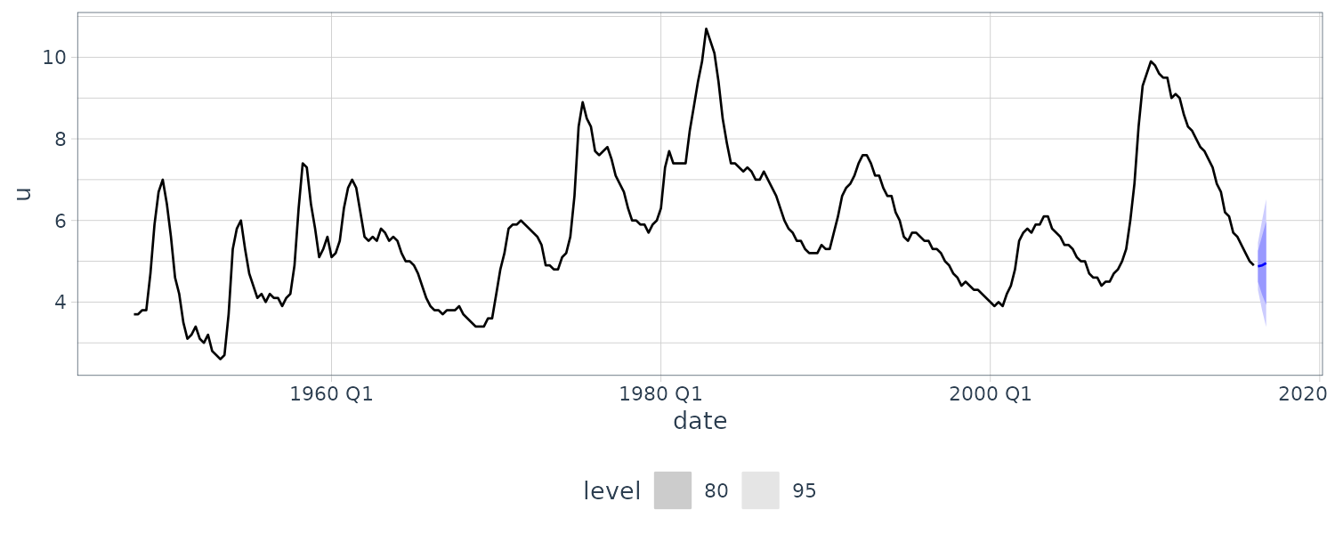
Note that the forecast variance we get is similar to dLagM, and recall the coefficients are similar too. So going forward while doing forecast, we would revert to using fable and using autocorrelation for the errors rather than using autoregressive terms.
Assumptions for Forecasting
Assumption 1
The time series \(y, x\) are stationary and weakly dependent.
Assumption 2
The conditional expectation is a linear function of a finite number of lags of \(y, x\):
\[\begin{aligned} E[y_{t}\mid I_{t-1}] &= \delta + \theta_{1}y_{t-1}+ \cdots + \theta_{p}y_{t-p} + \beta_{1}x_{t-1} + \cdots + \beta_{q}x_{t-1} \end{aligned}\]The error term is such that:
\[\begin{aligned} E[e_{t}\mid I_{t-1}] &= 0 \end{aligned}\]And not serially correlated:
\[\begin{aligned} E[e_{t}e_{s}\mid I_{t-1}] &= 0 \end{aligned}\] \[\begin{aligned} t &\neq s \end{aligned}\]For example, correlation between \(e_{t}, e_{t-1}\) implies that:
\[\begin{aligned} E[e_{t}\mid I_{t-1}] &= \rho e_{t-1}\\ E[y_{t}\mid I_{t-1}] &= \delta + \theta_{1}y_{t-1} + \rho e_{t-1} \end{aligned}\]This can be resolved by adding another lag of \(y\):
\[\begin{aligned} E[y_{t}\mid I_{t-1}] &= \delta + \theta_{1}y_{t-1} + \rho e_{t-1}\\ &= \delta(1 - \rho) + (\theta_{1} + \rho)y_{t-1} - \rho \theta_{1}y_{t-2} \end{aligned}\]The assumption that \(E[e_{t}\mid I_{t-1}] = 0\) does not mean that a past error \(e_{t-j}\) could not affect current and future values of \(x\). If \(x\) is a policy variable whose setting reacts to past values of \(e\) and \(y\), the least squares estimator is still consistent. However, correlation between \(e_{t}\) and past values of \(x\) must be uncorrelated.
Assumption 3
The errors are conditional homoskedastic:
\[\begin{aligned} \textrm{var}(e_{t}\mid I_{t-1}) &= \sigma^{2} \end{aligned}\]This assumption is needed for the traditional least squares standard errors to be valid and to compute the forecast standard errors.
Selecting Lag Lengths
How do we decide on \(p, q\)? There are a few ways to do this:
- Extend the lag lengths for \(y, x\) as long as their estimated coefficients are significantly different from 0.
- Choose \(p, q\) to minimize the AIC/BIC.
- Evaluate the out-of-sample forecasting performance of each \(p,q\) combination using a hold-out sample.
- To check for serial correlation in the error term.
Granger Causality
Granger causality refers to the ability of lags of one variable to contribute to the forecast of another variable. In this case the variable \(x\) “Granger cause” \(y\) if:
\[\begin{aligned} y_{t} &= \delta + \theta_{1}y_{t-1} + \cdots + \theta_{p}y_{t-p} + \beta_{0}x_{t} + \cdots \beta_{q}x_{t-q} + e_{t} \end{aligned}\]Or if variable \(x\) does not “Granger clause” \(y\) if:
\[\begin{aligned} E[y_{t}|y_{t-1}, y_{t-2}, \cdots, y_{t-p}, x_{t-1}, x_{t-2}, \cdots, x_{t-q}] &= E[y_{t}|y_{t-1}, y_{t-2}, \cdots, y_{t-p}] \end{aligned}\]To test for Granger Causality, we use the following hypothesis testing and running a F-test:
\[\begin{aligned} H_{0}: &\beta_{1} = 0, \cdots, \beta_{q} = 0\\ H_{1}: &\text{At least one }\beta_{i} \neq 0 \end{aligned}\]This can be done using the F-test.
Note that if x Granger causes y, it does not necessarily imply a direct causal relationship between x and y. It means that having information on past x values will improve the forecast for y. Any causal effect can be an indirect one.
Example: Does the Growth Rate Granger Cause Unemployment?
Recall:
\[\begin{aligned} \hat{U}_{t} &= 0.3616 + 1.5331 U_{t-1} - 0.5818 U_{t-2} - 0.04824 G_{t-1} \end{aligned}\]To calculate the F-statistic:
\[\begin{aligned} F &= t^{2}\\ &= \Bigg(\frac{0.04824}{\text{SE}(G_{t-1})}\Bigg)^{2}\\ &= \Bigg(\frac{0.04824}{0.01949}\Bigg)^{2}\\ &= 6.126 \end{aligned}\]We can calculate the F-value for \(F_{(0.95, 1, 267)}\) in R:
> qf(0.95, df1 = 1, df2 = 267)
3.876522
Or we could use anova() function:
fitR <- lm(
  u ~ lag(u) +
    lag(u, 2),
  data = usmacro
)

fitU <- lm(
  u ~ lag(u) +
    lag(u, 2) +
    lag(g),
  data = usmacro
)

> anova(fitU, fitR)
Analysis of Variance Table

Model 1: u ~ lag(u) + lag(u, 2) + lag(g)
Model 2: u ~ lag(u) + lag(u, 2)
  Res.Df    RSS Df Sum of Sq      F  Pr(>F)
1    267 22.753
2    268 23.276 -1  -0.52209 6.1264 0.01394 *
---
Signif. codes:  0 ‘***’ 0.001 ‘**’ 0.01 ‘*’ 0.05 ‘.’ 0.1 ‘ ’ 1
Since \(6.126 > 3.877\), we would reject the null hypothesis and conclude that \(G\) Granger causes \(U\).
If there is more than one lag:
\[\begin{aligned} \hat{U}_{t} &= \delta + \theta_{1}U_{t-1} + \theta_{2}U_{t-2} + \beta_{1}G_{t-1} + \beta_{2}G_{t-2} + \beta_{3}G_{t-3} + \beta_{4}G_{t-4} + e_{t} \end{aligned}\]Using anova() in R:
fitR <- lm(
  u ~ lag(u)
    + lag(u, 2) +
    lag(g),
  data = usmacro[3:nrow(usmacro), ]
)

fitU <- lm(
  u ~ lag(u) +
    lag(u, 2) +
    lag(g) +
    lag(g, 2) +
    lag(g, 3) +
    lag(g, 4),
  data = usmacro
)

> anova(
  fitU,
  fitR
)
Analysis of Variance Table

Model 1: u ~ lag(u) + lag(u, 2) + lag(g) + lag(g, 2) +
    lag(g, 3) + lag(g, 4)
Model 2: u ~ lag(u) + lag(u, 2) + lag(g)
  Res.Df    RSS Df Sum of Sq      F   Pr(>F)
1    262 21.302
2    265 22.738 -3   -1.4358 5.8865 0.000667 ***
---
Signif. codes:  0 ‘***’ 0.001 ‘**’ 0.01 ‘*’ 0.05 ‘.’ 0.1 ‘ ’ 1
Because anova require the same dataset, and the first 2 lags of the reduced model is not used, we need to subset the dataset.
The formula for F-statistic:
\[\begin{aligned} F &= \frac{Mean of squares between groups}{Mean of squares within groups}\\ &= \frac{\frac{SSE_{R} - SSE_{U}}{df_{R} - df_{U}}}{\frac{SSE_{U}}{df_{U}}} \end{aligned}\]Testing for Serially Correlated Errors
For the abscene of serial correlation, we require the conditional covariance between any two different errors to be 0:
\[\begin{aligned} E[e_{t}e_{s}\mid I_{t-1}] &= 0\\ t &\neq s \end{aligned}\]If the errors are serally correlated, then the usual least squares standard errors are invalid.
We will discuss 3 ways to test for serial correlated errors:
- Checking Correlogram
- Lagrange Multiplier Test
- Durbin-Watson Test
Checking the Correlogram of the Least Squares Residuals
We can check the correlogram for any autocorrelations that are significantly different from zero.
The kth order autocorrelation for the residuals is:
\[\begin{aligned} r_{k} &= \frac{\sum_{t=k+1}^{T}\hat{e}_{t}\hat{e}_{t-k}}{\sum_{t=1}^{T}\hat{e}_{t}^{2}} \end{aligned}\]For no correlation, ideally would like:
\[\begin{aligned} |r_{k}| < \frac{2}{\sqrt{T}} \end{aligned}\]Example: Checking the Residual Correlogram for the ARDL(2, 1) Unemployment Equation
fit <- lm(
  u ~ lag(u) +
    lag(u, 2) +
    lag(g),
  data = usmacro
)

usmacro$residuals <- c(NA, NA, resid(fit))

usmacro |>
  ACF(residuals) |>
  autoplot() +
  ggtitle("ACF") +
  theme_tq()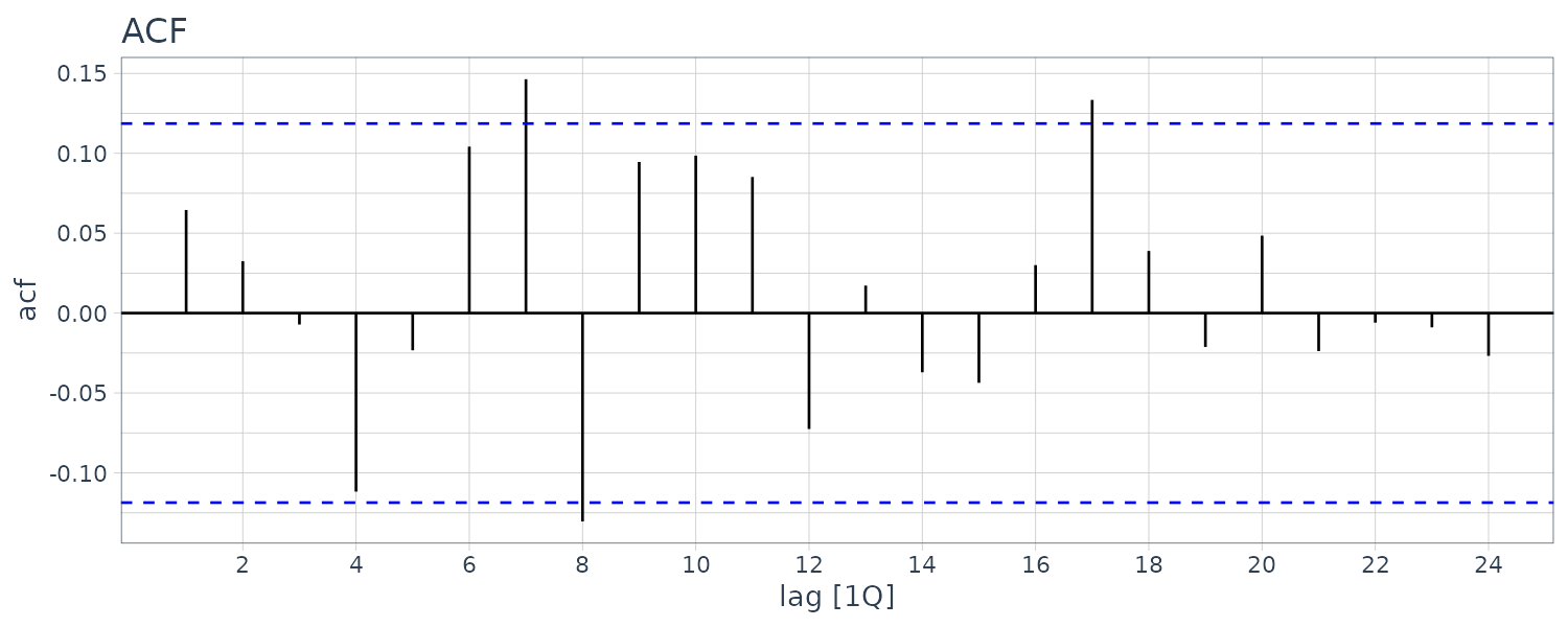
We can do this using fable as well:
fit <- usmacro |>
  model(
    ARIMA(
      u ~ lag(g) +
        pdq(2, 0, 0) +
        PDQ(0, 0, 0)
    )
  )

fit |>
  gg_tsresiduals() |>
  purrr::pluck(2) +
  theme_tq()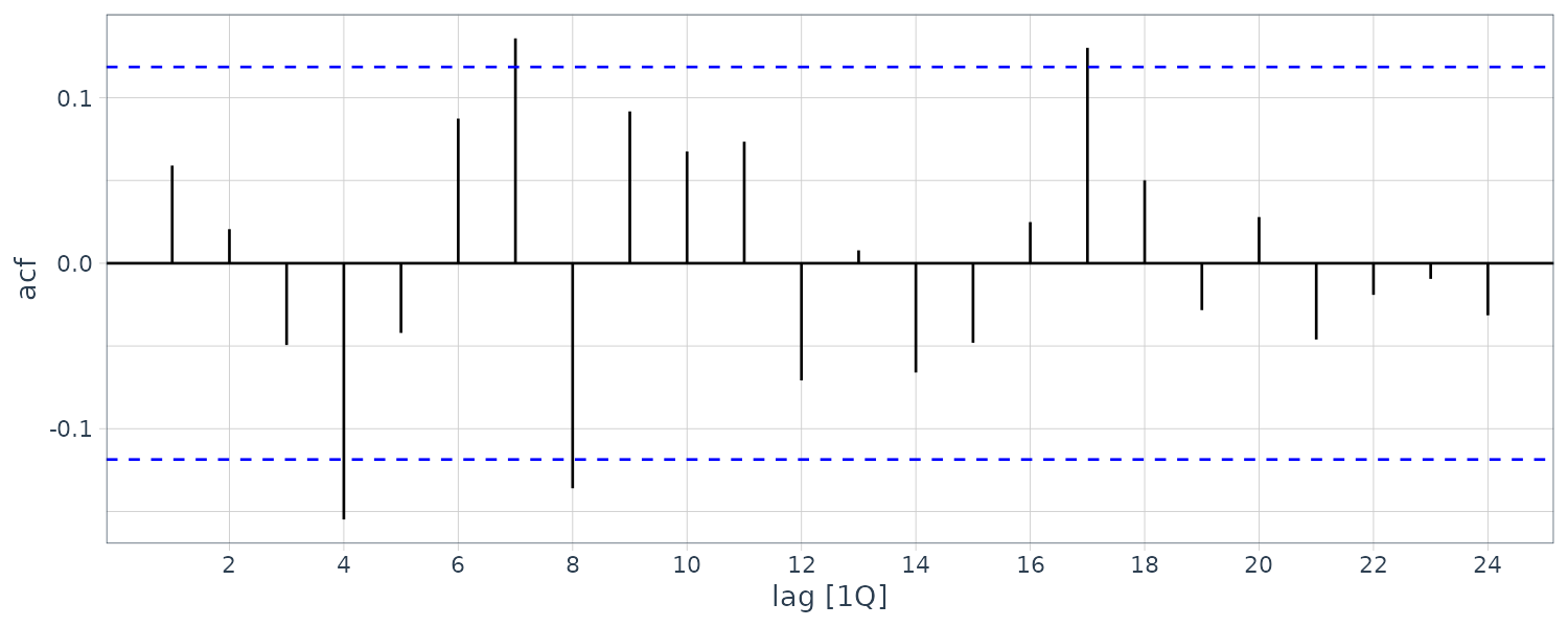
Example: Checking the Residual Correlogram for an ARDL(1, 1) Unemployment Equation
Suppose we omit \(U_{t-2}\). If \(U_{t-2}\) is an important predictor, it should lead to serial correlation in the errors. We can graph the correlogram to see this:
fit <- usmacro |>
  model(
    ARIMA(
      u ~ lag(g) +
        pdq(1, 0, 0) +
        PDQ(0, 0, 0)
    )
  )

fit |>
  gg_tsresiduals() |>
  purrr::pluck(2) +
  theme_tq()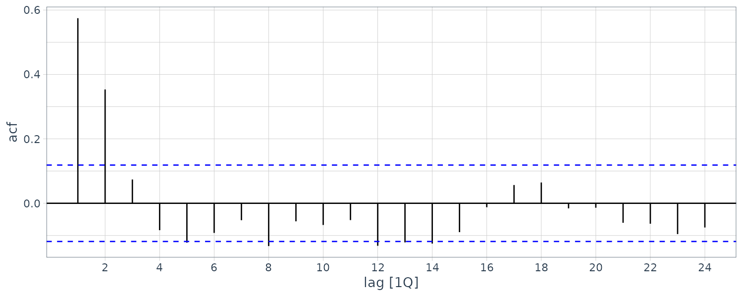
Example: Lagrange Multiplier Test
Also known as the Breusch-Godfrey test. It is based on the idea of Lagrange multiplier testing.
Consider the ARDL(1, 1) model:
\[\begin{aligned} y_{t} &= \delta + \beta_{1}x_{t-1} + \beta_{2}x_{t-2} + e_{t} \end{aligned}\]The null hypothesis is that the errors \(e_{t}\) are uncorrelated. To express this null hypothesis in terms of restrictions on one or more parameters, we can introduce a model for an alternative hypothesis, with that model describing the possible nature of any autocorrelation. We will consider a number of alternative models.
Testing for AR(1) Errors
In the first instance, we consider an alternative hypothesis that the errors are correlated through the AR(1) process:
\[\begin{aligned} e_{t} &= \rho e_{t-1} + v_{t} \end{aligned}\]Where the errors \(v_{t}\) are uncorrelated. Substituting \(e_{t}\) in the above equation:
\[\begin{aligned} y_{t} &= \delta + \theta_{1}y_{t-1} + \beta_{1}x_{t-1} + \rho e_{t-1} + v_{t} \end{aligned}\]We can draft the the hypothesis as:
\[\begin{aligned} H_{0}:&\ \rho = 0\\ H_{1}:&\ \rho \neq 0 \end{aligned}\]One way is to regress \(y_{t}\) on \(y_{t-1}, x_{t-1}, e_{t-1}\) and test for the significance of the coefficient of \(\hat{e}_{t-1}\) as we can’t observe \(e_{t-1}\) and to then use a t- or F-test to test the significance of the coefficient of \(e_{t-1}\).
A second way is to derive the relevant auxiliary regression for the autocorrelation LM test:
\[\begin{aligned} y_{t} &= \delta + \theta y_{t-1} + \beta_{1}x_{t-1} + \rho \hat{e}_{t-1} + v_{t} \end{aligned}\]Note that:
\[\begin{aligned} y_{t} &= \hat{y}_{t} + \hat{e}_{t}\\ &= \hat{\delta}+ \hat{\theta}_{1}y_{t-1} + \hat{\delta}_{1}x_{t-1} + \hat{e}_{t} \end{aligned}\]Subsitute into the original equation, we get:
\[\begin{aligned} \hat{\delta}_{t} + \hat{\theta}_{1}y_{t-1} + \hat{\beta}_{1}x_{t-1} + \hat{e}_{t} &= \delta + \theta y_{t-1} + \beta_{1}x_{t-1} + \rho \hat{e}_{t-1} + v_{t} \end{aligned}\]Rearranging the equation yields the auxiliary regression:
\[\begin{aligned} \hat{e}_{t} &= (\delta - \hat{\delta}) + (\theta_{1} - \hat{\theta}_{1})y_{t-1} + (\beta - \hat{\beta}_{1})x_{t-1} + \rho\hat{e}_{t-1} + v_{t}\\ &= \gamma_{1} + \gamma_{2}y_{t-1} + \gamma_{3}x_{t-1} + \rho\hat{e}_{t-1} + v_{t} \end{aligned}\] \[\begin{aligned} \gamma_{1} &= \delta - \hat{\delta}\\ \gamma_{2} &= \theta_{1} - \hat{\theta}_{1}\\ \gamma_{3} &= \delta_{1}- \hat{\delta}_{1} \end{aligned}\]Because \(\delta - \hat{\delta}, \theta_{1} - \hat{\theta}_{1}, \beta - \hat{\beta}_{1}\) are centered around zero, if there is significant explanatory power, it will come from \(\hat{e}_{t-1}\).
If \(H_{0}\) is true, then the LM has an approximately \(\chi_{(1)}^{2}\) distribution.
Testing for MA(1) Errors
The alternative hypothesis in this case is modeled using the MA(1) process:
\[\begin{aligned} e_{t} &= \phi v_{t-1} + v_{t} \end{aligned}\]Resulting in the following ARDL(1, 1) model:
\[\begin{aligned} y_{t} &= \delta + \theta_{1}y_{t-1} + \beta_{1}x_{t-1} + \phi v_{t-1} + v_{t} \end{aligned}\]The hypothesis would be:
\[\begin{aligned} H_{0}:&\ \phi = 0\\ H_{1}:&\ \phi \neq 0 \end{aligned}\]Testing for Higher Order AR or MA Errors
The LM test can be extended to alternative hypotheses in terms of higher order AR or MA models.
For example for an AR(4) model:
\[\begin{aligned} e_{t} &= \psi_{1}e_{t-1} + \psi_{2}e_{t-2} + \psi_{3}e_{t-3} + \psi_{4}e_{t-4} + v_{t} \end{aligned}\]And MA(4) model:
\[\begin{aligned} e_{t} &= \phi_{1}v_{t-1} + \phi_{2}v_{t-2} + \phi_{3}v_{t-3} + \phi_{4}v_{t-4} + v_{t} \end{aligned}\]AR(4) hypothesis:
\[\begin{aligned} H_{0}:&\ \psi_{1} = 0, \psi_{2} = 0, \psi_{3} = 0, \psi_{4} = 0\\ H_{1}:&\ \text{at least one } \psi_{i} \text{ is nonzero} \end{aligned}\] \[\begin{aligned} H_{0}:&\ \phi_{1} = 0, \phi_{2} = 0, \phi_{3} = 0, \phi_{4} = 0\\ H_{1}:&\ \text{at least one } \phi_{i} \text{ is nonzero} \end{aligned}\]The alternative auxillary equations will be::
\[\begin{aligned} \hat{y}_{t} &= \gamma_{1} + \gamma_{2}y_{t-1} + \gamma_{3}x_{t-1} + \psi_{1}\hat{e}_{t-1} + \psi_{2}\hat{e}_{t-2} +\psi_{3}\hat{e}_{t-3} +\psi_{4}\hat{e}_{t-4} + v_{t} \end{aligned}\]And MA(4) model:
\[\begin{aligned} \hat{e}_{t} &= \gamma_{1} + \gamma_{2}y_{t-1} + \gamma_{3}x_{t-1} + \phi_{1}\hat{e}_{t-1} + \phi_{2}\hat{e}_{t-2} +\phi_{3}\hat{e}_{t-3} +\phi_{4}\hat{e}_{t-4} + v_{t} \end{aligned}\]When \(H_{0}\) is true, the LM statistic would have a \(\chi_{(4)}^{2}\) distribution.
Durbin-Watson Test
Durbin-Watson test doesn’t require large sample approximation. The standard test is:
\[\begin{aligned} H_{0}:&\ \rho = 0\\ H_{1}:&\ \rho \neq 0 \end{aligned}\]For the AR(1) error model:
\[\begin{aligned} e_{t} &= \rho e_{t-1} + v_{t} \end{aligned}\]However it is not applicable when there are lagged dependent variables.
Both Ljung-Box and Durbin Watson are used roughly for the same purpose i.e. to check the autocorrelation in a data series. While Ljung-Box can be used for any lag value, Durbin Watson can be used just for the lag of 1.
Time-Series Regressions for Policy Analysis
In the previous section, our main focus was to estimate the AR or ARDL condition expectation:
\[\begin{aligned} E[y_{t}\mid I_{t-1}] &= \delta + \theta_{1}y_{t-1} + \cdots + \theta_{p}y_{t-p} + \delta_{1}x_{t-1} + \cdots + \delta_{q}x_{t-1} \end{aligned}\]We were not concerned with the interpretation of individual coefficients, or with omitted variables. Valid forecasts could be obtained from either of the models or one that contains other explanatory variables and their lags. Moreover, because we were using past data to forecast the future, a current value of x was not included in the ARDL model.
Models for policy analysis differ in a number of ways. The individual coeffcients are of interest because they might have a causal interpretation, telling us how much the average outcome of a dependent variable changes when an explanatory variable and its lags change.
For example, central banks who set interest rates are concerned with how a change in the interest rate will affect inflation, unemployment, and GDP growth, now and in the future. Because we are interested in the current effect of a change, as well as future effects, the current value of explanatory variables can appear in distributed lag or ARDL models. In addition, omitted variables can be a problem if they are correlated with the included variables because then the coefficients may not reflect causal effects.
Interpreting a coefficient as the change in a dependent variable caused by a change in an explanatory variable:
\[\begin{aligned} \beta_{k} &= \frac{\partial E[y_{t}\mid \textbf{x}_{t}]}{\partial x_{tk}} \end{aligned}\]Recall that \(\mathbf{X}\) denotes all observations in all time periods and the following strict exogeneity condition:
\[\begin{aligned} E[e_{t}\mid \textbf{X}] &= 0 \end{aligned}\]Implies that there are no lagged dependent variables on the RHS, thus ruling out ARDL models.
And the absence of serial correlation in the errors:
\[\begin{aligned} \text{cov}(e_{t}, e_{s}\mid \mathbf{X}) &= 0 \end{aligned}\] \[\begin{aligned} t &\neq s \end{aligned}\]Means that the errors are uncorrelated with future x values, an assumption that would be violated if x was a policy variable, such as the interest rate, whose setting was influenced by past values of y, such as the inflation rate. The absence of serial correlation implies that variables omitted from the equation, and whose effect is felt through the error term, must not be serially correlated.
In the general framework of an ARDL model, the contemporaneous exogeneity assumption can be written as:
\[\begin{aligned} E[e_{t}\mid I_{t}] &= 0 \end{aligned}\]Feedback from current and past \(y\) to future \(x\) is possible under this assumption.
For the OLS standard errors to be valid for large sample inference, the serially uncorrelated error assumption:
\[\begin{aligned} \text{cov}(e_{t}, e_{s}\mid \mathbf{X}) \end{aligned}\]Can be weakened to:
\[\begin{aligned} \text{cov}(e_{t}, e_{s}\mid I_{t}) \end{aligned}\]Finite Distributed Lag Models (FDL)
Suppose we are interested in the impact of current and past values of \(x\):
\[\begin{aligned} y_{t} &= \alpha + \beta_{0}x_{t} + \beta_{1}x_{t - 1} + \cdots + + \beta_{q}x_{t-1} + e_{t} \end{aligned}\]It is called finite distributed lag because \(x\) cuts off after q lags and distributed because the impact of change in \(x\) is distributed over future time periods.
Once \(q\) lags of \(x\) have been included in the equation, further lags of \(x\) will not have an impact on \(y\).
For the coefficients \(\beta_{k}\) to represent causal effects, the errors must not be correlated with the current and all past values of \(x\):
\[\begin{aligned} E[e_{t}|x_{t}, x_{t-1}, \cdots] &= 0 \end{aligned}\]It then follows that:
\[\begin{aligned} E[y_{t}\mid x_{t}, x_{t-1}, \cdots] &= \alpha + \beta_{0}x_{t} + \beta_{1}x_{t - 1} + \cdots + + \beta_{q}x_{t-1}\\ &= E[y_{t}\mid x_{t}, x_{t-1}, \cdots, x_{t-q}]\\ &= E[y_{t}\mid \textbf{x}_{t}] \end{aligned}\]Given this assumption, a lag-coefficient \(\beta_{s}\) can be interpreted as the change in \(E[y_{t}\mid \textbf{x}_{t}]\) when \(x_{t-s}\) changes by 1 unit, given \(x\) held constant in other periods:
\[\begin{aligned} \beta_{s} &= \frac{\partial E[y_{t}|\textbf{x}_{t}]}{\partial x_{t-s}} \end{aligned}\]Also applicable for future forecast:
\[\begin{aligned} \beta_{s} &= \frac{\partial E[y_{t+s}|\textbf{x}_{t}]}{\partial x_{t}} \end{aligned}\]To show how the change propagate across time, suppose that \(x_{t}\) is increased by 1 unit and returned to its original level in subsequent periods. The immediate effect will be an increase in \(y_{t}\) by \(\beta_{0}\) units. On period later, \(y_{t+1}\) will be increased by \(\beta_{1}\) units and q periods later, \(y_{t+q}\) will be increased by \(\beta_{q}\) and finally return to the original level by \(y_{t+q+1} = y_{t}\). This is known as the interim multiplier.
If the change in \(x\) by 1 is sustained throughout the period, the immediate effect would be an increased by \(\beta_{0}\), followed by \(\beta_{0} + \beta_{1}\), until \(\sum_{s = 0}^{q}\beta_{s}\) and held there. This is known as the total multiplier.
For example \(y\) could be the inflation rate, and \(x\) the interest rate. So what the equation is saying is inflation at \(t\) depends on current and past interest rates.
Finite Distributed Lags models can be used in forecasting or policy analysis. For policy analysis, the central bank might want to know who inflation will react given a change in the current interest rate.
Okun’s Law Example
We are going to illustrate FDL by using an Okun’s Law example. The basic Okun’s Law shows the relationship between unemployment growth and GDP growth:
\[\begin{aligned} U_{t} - U_{t-1} &= -\gamma(G_{t} - G_{N}) \end{aligned}\]Where \(U_{t}\) is the unemployment rate in period \(t\), and \(G_{t}\) is the growth rate of output in period \(t\), and \(G_{N}\) is the neutral growth rate which we would assume to be constant. We would expect \(0 < \gamma < 1\), reflecting the output growth leads to less than one-to-one change in unemployment.
Rewriting the relationship and adding an error term:
\[\begin{aligned} \Delta U_{t} &= \gamma G_{N} -\gamma G_{t} + e_{t}\\ &= \alpha + \beta_{0}G_{t} + e_{t} \end{aligned}\]Expecting that changes in output are likely to have a distributed-lag effect on unemployment (possibly due to employment being sticky):
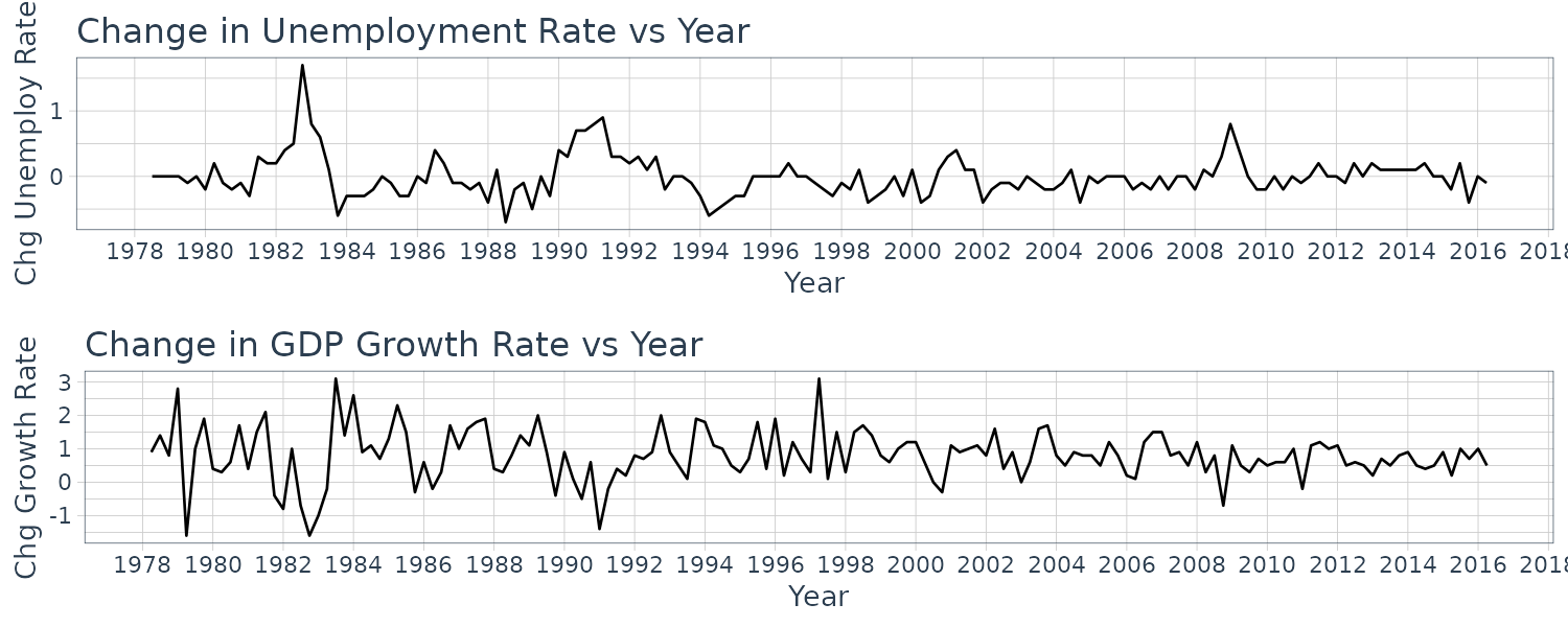
\[\begin{aligned} \Delta U_{t} &= \alpha + \beta_{0}G_{t} + \beta_{1}G_{t - 1} + \cdots + \beta_{q}G_{t-q} + e_{t} \end{aligned}\]To illustrate this, we would use the okun5_aus data which contain the quarterly Australian data on unemployment and percentage change in GDP.
Our purpose is not to forecast unemployment but to investigate the lagged responses of unemployment to growth in the economy. The normal growth rate \(G_{N}\) is the rate of output growth needed to maintain a constant unemployment rate. It is equal to the sum of labor force growth and labor productivity growth. We expect \(0 < \gamma < 1\), reflecting that output growth leads to less than one-to-one adjustments in unemployment.
Plotting the change in unemployment rate vs GDP:
okun5_aus$date <- as.Date(
  okun5_aus$dateid01,
  format = "%m/%d/%Y"
) |>
  yearquarter()

okun5_aus <- okun5_aus |>
  as_tsibble(index = date)

okun5_aus <- okun5_aus |>
  mutate(
    du = c(NA, diff(u))
  )

plot_grid(
  okun5_aus |>
    autoplot(du) +
    ylab("Chg Unemploy Rate") +
    xlab("Year") +
    ggtitle("Change in Unemployment Rate vs Year") +
    scale_x_yearquarter(
      date_breaks = "2 years",
      date_labels = "%Y"
    ) +
    theme_tq(),
  okun5_aus |>
    autoplot(g) +
    ylab("Chg Growth Rate") +
    xlab("Year") +
    ggtitle("Change in GDP Growth Rate vs Year") +
    scale_x_yearquarter(
      date_breaks = "2 years",
      date_labels = "%Y"
    ) +
    theme_tq(),
  ncol = 1
)
We fit for \(q = 5\):
fit <- lm(
  du ~ g +
    lag(g, 1) +
    lag(g, 2) +
    lag(g, 3) +
    lag(g, 4) +
    lag(g, 5),
  data = okun5_aus
)

> summary(fit)
Call:
lm(formula = du ~ g + lag(g, 1) + lag(g, 2) + lag(g, 3) +
    lag(g, 4) + lag(g, 5), data = okun5_aus)

Residuals:
     Min       1Q   Median       3Q      Max
-0.68569 -0.13548 -0.00477  0.10739  0.94163

Coefficients:
            Estimate Std. Error t value            Pr(>|t|)
(Intercept)  0.39298    0.04493   8.746 0.00000000000000601 ***
g           -0.12872    0.02556  -5.037 0.00000142519603254 ***
lag(g, 1)   -0.17207    0.02488  -6.915 0.00000000014967724 ***
lag(g, 2)   -0.09320    0.02411  -3.865            0.000169 ***
lag(g, 3)   -0.07260    0.02411  -3.012            0.003079 **
lag(g, 4)   -0.06363    0.02407  -2.644            0.009127 **
lag(g, 5)    0.02317    0.02398   0.966            0.335547
---
Signif. codes:  0 ‘***’ 0.001 ‘**’ 0.01 ‘*’ 0.05 ‘.’ 0.1 ‘ ’ 1

Residual standard error: 0.2258 on 141 degrees of freedom
  (5 observations deleted due to missingness)
Multiple R-squared:  0.5027,	Adjusted R-squared:  0.4816
F-statistic: 23.76 on 6 and 141 DF,  p-value: < 0.00000000000000022
All coefficients of \(G\) except for \(G_{t-5}\) are significant at the 5% level. Excluding lag 5 we get:
fit <- lm(
  du ~ g +
    lag(g, 1) +
    lag(g, 2) +
    lag(g, 3) +
    lag(g, 4),
  data = okun5_aus
)

> summary(fit)
Call:
lm(formula = du ~ g + lag(g, 1) + lag(g, 2) + lag(g, 3) +
    lag(g, 4), data = okun5_aus)

Residuals:
     Min       1Q   Median       3Q      Max
-0.67310 -0.13278 -0.00508  0.10965  0.97392

Coefficients:
            Estimate Std. Error t value             Pr(>|t|)
(Intercept)  0.40995    0.04155   9.867 < 0.0000000000000002 ***
g           -0.13100    0.02440  -5.369      0.0000003122555 ***
lag(g, 1)   -0.17152    0.02395  -7.161      0.0000000000388 ***
lag(g, 2)   -0.09400    0.02402  -3.912             0.000141 ***
lag(g, 3)   -0.07002    0.02391  -2.929             0.003961 **
lag(g, 4)   -0.06109    0.02384  -2.563             0.011419 *
---
Signif. codes:  0 ‘***’ 0.001 ‘**’ 0.01 ‘*’ 0.05 ‘.’ 0.1 ‘ ’ 1

Residual standard error: 0.2251 on 143 degrees of freedom
  (4 observations deleted due to missingness)
Multiple R-squared:  0.4988,	Adjusted R-squared:  0.4813
F-statistic: 28.46 on 5 and 143 DF,  p-value: < 0.00000000000000022
So what does the estimate for \(q = 4\) tells us? A 1% increase in the growth rate leads to a fall in the expected unemployment rate of 0.13% in the curent quarter, a fall of 0.17% in the next quarter, and 0.09%, 0.07% and 0.06% in the next 2 to 4 quarters.
The interim multipliers, which give the effect of a sustained increase in the growth rate of 1% are -0.30% in the first quarter, -0.40% for 2 quarters, -0.47% for 3 quarters, and -0.53% for 4 quarters.
An estimate of \(\gamma\), the total effect of a change in output growth in a year:
\[\begin{aligned} \hat{\gamma} &= -\sum_{s=0}^{4}b_{s}\\ &= 0.5276\% \end{aligned}\]An estimate of the normal growth rate that is needed to maintain a constant unemployment rate for a quarter:
\[\begin{aligned} \hat{G}_{n} &= \frac{\hat{\alpha}}{\hat{\gamma}}\\ &= \frac{0.4100}{0.5276}\\ &= 0.78\% \end{aligned}\]Two of the FDL assumptions commonly violated are that the error term is not autocorrelated and the error term is homoskedastic:
\[\begin{aligned} \text{cov}(e_{t}, e_{s}\mid \mathbf{x}_{t}, \mathbf{x}_{s}) &= E[e_{t}e_{s}\mid \mathbf{x}_{t}, \mathbf{x}_{s}]\\ &= 0\\[5pt] \text{var}(e_{t}\mid \mathbf{x}_{t}, \mathbf{x}_{s}) &= \sigma^{2} \end{aligned}\]However, it is still possible to use the OLS estimator with the HAC standard errors if the above 2 assumptions are violated as we cover in the next section.
Heteroskedasticity and Autocorrelation Consistent (HAC) Standard Errors
First let us consider the simple regression model where we drop the lagged variables:
\[\begin{aligned} y_{t} &= \alpha + \beta_{2}x_{t} + e_{t} \end{aligned}\]First we note that:
\[\begin{aligned} b_{2} &= \frac{\sum_{t}(x_{t} - \bar{x})(y_{t} - \bar{y})}{\sum_{t}(x_{t}- \bar{x})^{2}}\\[5pt] &= \frac{\sum_{t}y_{t}(x_{t} - \bar{x})- \bar{y}\sum_{t}(x_{t} - \bar{x})}{\sum_{t}(x_{t}- \bar{x})^{2}}\\[5pt] &= \frac{\sum_{t}y_{t}(x_{t} - \bar{x})- 0}{\sum_{t}(x_{t}- \bar{x})^{2}}\\[5pt] &= \frac{\sum_{t}(x_{t} - \bar{x})y_{t}}{\sum_{t}(x_{t}- \bar{x})^{2}}\\[5pt] &= \sum_{t}\frac{x_{t}- \bar{x}}{\sum_{t}(x_{t} - \bar{x})^{2}}y_{t}\\[5pt] &= \sum_{t}w_{t}y_{t} \end{aligned}\]The least squares estimator can also be written as:
\[\begin{aligned} b_{2} &= \sum_{t}w_{t}y_{t}\\[5pt] &= \sum_{t}w_{t}(\beta_{2}x_{t} + e_{t})\\[5pt] &= \beta_{2}\sum_{t}w_{t} + \sum_{t}w_{t}e_{t}\\[5pt] &= \beta_{2} + \sum_{t}w_{t}e_{t}\\[5pt] &= \beta_{2} + \frac{\frac{1}{T}\sum_{t}(x_{t} - \bar{x})e_{t}}{\frac{1}{T}\sum_{t}(x_{t} - \bar{x})^{2}}\\[5pt] &= \beta_{2} + \frac{\frac{1}{T}\sum_{t}(x_{t} - \bar{x})e_{t}}{s_{x}^{2}} \end{aligned}\]When \(e_{t}\) is homoskedastic and uncorrelated, we can take the variance of the above and show that:
\[\begin{aligned} \text{var}(b_{2}|\mathbf{X}) &= \frac{\sigma_{e}^{2}}{\sum_{t=1}^{T}(x_{t} - \bar{x})^{2}}\\[5pt] &= \frac{\sigma_{e}^{2}}{Ts_{x}^{2}} \end{aligned}\]For a result that is not conditional on \(\mathbf{X}\), we obtained the large sample approximate variance from the variance of its asymptotic distribution:
\[\begin{aligned} \mathrm{var}(b_{2}) &= \frac{\sigma_{e}^{2}}{T\sigma_{x}^{2}}\\ s_{x}^{2} &\overset{p}{\rightarrow}\sigma_{x}^{2} \end{aligned}\]Hence given large sample approximate variance we get the following result:
\[\begin{aligned} \text{var}(b_{2}) &= \frac{\sigma_{e}^{2}}{T\sigma_{x}^{2}} \end{aligned}\]But what if both \(b_{2}\) and \(e_{t}\) are heteroskedastic and autocorrelated? Replacing \(s_{x}^{2}\) with \(\sigma_{x}^{2}\) and \(\bar{x}\) with \(\mu_{x}\):
\[\begin{aligned} \text{var}(b_{2}) &= \textrm{var}\Bigg(\frac{\frac{1}{T}\sum_{t=1}^{T}(x_{t} - \mu_{x})e_{t}}{\sigma_{x}^{2}}\Bigg)\\[5pt] &= \frac{1}{T^{2}(\sigma_{x}^{2})^{2}}\textrm{var}\Big(\sum_{t}^{T}q_{t}\Big)\\[5pt] &= \frac{1}{T^{2}(\sigma_{x}^{2})^{2}}\Bigg(\sum_{t=1}^{T}\textrm{var}(q_{t}) + 2\sum_{t=1}^{T-1}\sum_{s=1}^{T-t}\textrm{cov}(q_{t}, q_{t+s})\Bigg)\\[5pt] &= \frac{\sum_{t=1}^{T}\textrm{var}(q_{t})}{T^{2}(\sigma_{x}^{2})^{2}}\Bigg(1 + \frac{2\sum_{t=1}^{T-1}\sum_{s=1}^{T-t}\textrm{cov}(q_{t}, q_{t+s})}{\sum_{t=1}^{T}\text{var}(q_{t})}\Bigg) \end{aligned}\] \[\begin{aligned} q_{t} &= (x_{t}- \mu_{x})e_{t} \end{aligned}\]HAC standard errors are obtained by considering estimators for the quantity outside the big brackets and the quantity inside the big brackets. For the quantity outside the brackets, first note that \(q_{t}\) has a zero mean and:
\[\begin{aligned} \hat{\textrm{var}}_{HCE}(b_{2}) &= \frac{\sum_{t=1}^{T}\textrm{var}(\hat{q}_{t})}{T^{2}(\sigma_{x}^{2})^{2}}\\[5pt] &= \frac{T\sum_{t=1}^{T}(x_{t} - \bar{x})^{2}\hat{e}_{t}^{2}}{(T-K)\Big(\sum_{t=1}^{T}(x_{t} - \bar{x})^{2}\Big)^{2}}\\[5pt] \hat{\textrm{var}}(\hat{q}_{t}) &= \frac{\sum_{t=1}^{T}(x_{t} - \bar{x})^{2}\hat{e}_{t}^{2}}{T-k}\\[5pt] (s_{x}^{2})^{2} &= \Big(\frac{\sum_{t=1}^{T}(x_{t} - \bar{x})^{2}}{T}\Big)^{2} \end{aligned}\]Note that the extra \(T\) in the numerator is what due to the heteroskedasticity.
The quantity outside the brackets is the large sample unconditional variance of \(b_{0}\) when there is heteroskedasticity but no autocorrelation.
To get the variance estimator for least squares that is consistent in the presence of both heteroskedasticity and autocorrelation, we need to multiply the HCE variance estimator by the quantity inside the bracket which we will denote as \(g\):
\[\begin{aligned} g &= 1 + \frac{2\sum_{t=1}^{T-1}\sum_{s=1}^{T-t}\textrm{cov}(q_{t}, q_{t+s})}{\sum_{t=1}^{T}\text{var}(q_{t})}\\[5pt] &= 1 + \frac{2\sum_{t=1}^{T-1}(T-s)\sum_{s=1}^{T-s}\textrm{cov}(q_{t}, q_{t+s})}{T\text{var}(q_{t})}\\[5pt] &= 1 + 2\sum_{s=1}^{T-1}\Big(\frac{T-s}{T}\Big)\tau_{s} \end{aligned}\] \[\begin{aligned} \tau_{s} &= \frac{\textrm{cov}(q_{t}, q_{t+s})}{\textrm{var}(q_{t})}\\[5pt] &= \textrm{corr}(q_{t}, q_{t+s}) \end{aligned}\]As we can see \(\tau_{s}\) is the autocorrelation. So when there is no serial correlation:
\[\begin{aligned} \tau_{s} &= 0\\ g &= 1 + 0\\ &= 1 \end{aligned}\]To obtain a consistent estimator for \(g\), the summation is truncated at a lag much smaller than \(T\). The autocorrelation lags beyond that are taken as zero. For example, if 5 autocorrelations are used, the corresponding estimator is:
\[\begin{aligned} \hat{g}&= 1 + 2 \sum_{s=1}^{5}\Big(\frac{6-s}{6}\Big)\hat{\tau}_{s} \end{aligned}\]Note that different software packages might yield different HAC standard errors as they use different estimation of the number of lags.
Finallly, given a suitable estimator \(\hat{g}\), the large sample estimator for the variance of \(b_{2}\), allowing for both heteroscedasticity and autocorrelation in the errors (HAC) is:
\[\begin{aligned} \hat{\textrm{var}}_{HAC}(b_{2}) &= \hat{\textrm{var}}_{HCE}(b_{2}) \times \hat{g} \end{aligned}\]Example: A Phillips Curve
The Phillips curve describes the relationship between inflation and unemployment:
\[\begin{aligned} \text{INF}_{t} &= \text{INF}_{t}^{E}- \gamma(U_{t} - U_{t-1}) \end{aligned}\]\(\text{INF}_{t}^{E}\) is the expection inflation for period \(t\).
The hypothesis is that falling levels of unemployment will cause higher inflation from excess demand for labor that drives up wages and vice versa for rising levels of unemployment.
Written as simple regression model:
\[\begin{aligned} \text{INF}_{t} &= \alpha + \beta_{1}\Delta U_{t} + e_{t} \end{aligned}\]Using the quarterly Australian data phillips5_aus:
phillips5_aus$date <- as.Date(
  phillips5_aus$dateid01,
  format = "%m/%d/%Y"
) |>
  yearquarter()

phillips5_aus <- phillips5_aus |>
  as_tsibble(index = date)

phillips5_aus <- phillips5_aus |>
  mutate(
    du = c(NA, diff(u))
  )
Graphing the inflation rate:
phillips5_aus |>
  autoplot(inf) +
  ylab("Inflation Rate") +
  xlab("Year") +
  ggtitle("Inflation Rate vs Year") +
  scale_x_yearquarter(
    date_breaks = "2 years",
    date_labels = "%Y"
  ) +
  theme_tq()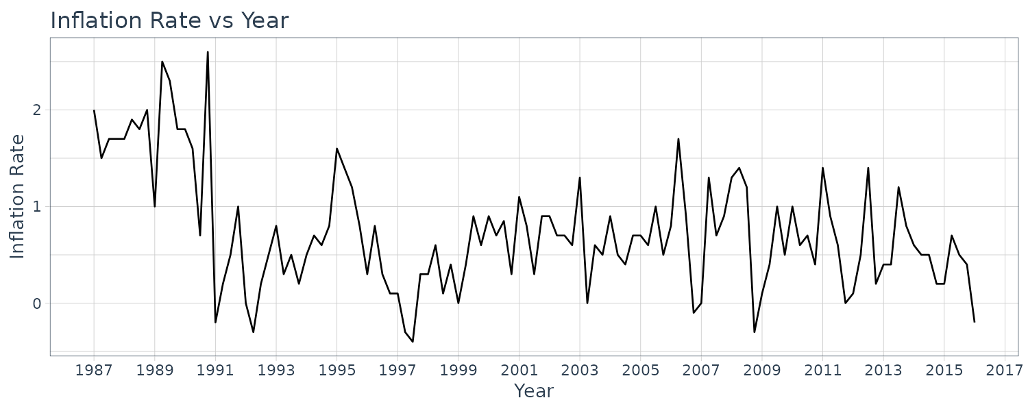
Fitting the model and graphing the residuals:
fit <- lm(inf ~ du, data = phillips5_aus)

> summary(fit)
Call:
lm(formula = inf ~ du, data = phillips5_aus)

Residuals:
    Min      1Q  Median      3Q     Max
-1.2115 -0.3919 -0.1121  0.2683  2.1473

Coefficients:
            Estimate Std. Error t value Pr(>|t|)
(Intercept)  0.73174    0.05606  13.053   <2e-16 ***
du          -0.39867    0.20605  -1.935   0.0555 .
---
Signif. codes:  0 ‘***’ 0.001 ‘**’ 0.01 ‘*’ 0.05 ‘.’ 0.1 ‘ ’ 1

Residual standard error: 0.6043 on 115 degrees of freedom
Multiple R-squared:  0.03152,	Adjusted R-squared:  0.0231
F-statistic: 3.743 on 1 and 115 DF,  p-value: 0.05547

phillips5_aus |>
  ACF(fit$residuals) |>
  autoplot() +
  ggtitle("ACF") +
  theme_tq()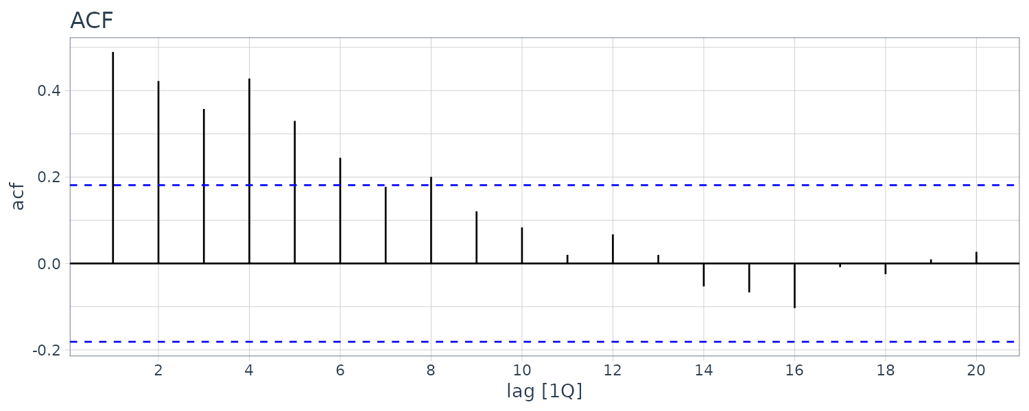
To calculate the HCE in R:
norms <- (phillips5_aus$du - mean(phillips5_aus$du))^2
T <- nrow(phillips5_aus)

hac <- (T * sum(norms * fit$residuals^2)) /
  ((T - 2)*(sum(norms)^2))

> sqrt(hac)
[1] 0.2631565
Contrasts that with OLS SE of 0.2061.
To adjust for autocorrelation and heteroskedasticity (HAC):
acfs <- phillips5_aus |>
  ACF(fit$residuals * norms) |>
  pull(acf)

tmp <- 0
T <- 7
for (i in 1:T) {
  tmp <- tmp + (T - i)/T * acfs[i]
}
tmp
g <- 1 + 2*tmp

> sqrt(hac * g)
[1] 0.2895455
Estimation with AR(1) Errors
Using least squares with HAC standard errors overcomes the negative consequences that autocorrelated errors have for least squares standard errors. However, it does not address the issue of finding an estimator that is better in the sense that it has a lower variance. One way to proceed is to make an assumption about the model that generates the autocorrelated errors and to derive an estimator compatible with this assumption. In this section, we examine how to estimate the parameters of the regression model when one such assumption is made, that of AR(1) errors.
Consider the simple regression model:
\[\begin{aligned} y_{t} &= \alpha + \beta_{2}x_{t} + e_{t} \end{aligned}\]The AR(1) error model:
\[\begin{aligned} e_{t} &= \rho e_{t-1} + v_{t} \end{aligned}\] \[\begin{aligned} |\rho| &< 1 \end{aligned}\]The errors \(v_{t}\) are assumed to be uncorrelated, with zero mean and constant variances:
\[\begin{aligned} E[v_{t}\mid x_{t}, x_{t-1}, \cdots] &= 0\\ \textrm{var}(v_{t}\mid x_{t}) &= \sigma_{v}^{2}\\ \textrm{cov}(v_{t}, v_{s}) &= 0 \end{aligned}\]It can further be shown that this result in the following properties for \(e_{t}\):
\[\begin{aligned} E[e_{t}] &= 0 \end{aligned}\] \[\begin{aligned} \sigma_{e}^{2} &= \frac{\sigma_{v}^{2}}{1 - \rho^{2}} \end{aligned}\] \[\begin{aligned} \rho_{k} &= \rho^{k} \end{aligned}\]Recall that AR(1) error model leads to the following equation:
\[\begin{aligned} y_{t} &= \alpha(1 - \rho) + \rho y_{t-1} + \beta_{0}x_{t} - \rho \beta_{0}x_{t-1} + v_{t} \end{aligned}\]But now we have turned the coefficient of \(x_{t-1}\) to be \(-\rho\beta_{0}\) causing the whole equation to be nonlinear. To obtain estimates, we would need to employ numerical methods.
To introduce an alternative estimator for the AR(1) error model, we rewrite:
\[\begin{aligned} y_{t} - \rho y_{t-1} &= \alpha(1 - \rho) + \beta_{0}x_{t} - \rho \beta_{0}x_{t-1} + v_{t} \end{aligned}\] \[\begin{aligned} y_{t}^{*} &= \alpha^{*} + \beta_{0}x_{t}^{*} + v_{t} \end{aligned}\] \[\begin{aligned} y_{t}^{*} &= y_{t} - \rho y_{t-1}\\ \alpha^{*} &= \alpha(1 - \rho)\\ x^{*} &= x_{t} - \rho x_{t-1} \end{aligned}\]OLS can then be applied and if \(\rho\) is known, then the original intercept can be recovered:
\[\begin{aligned} \hat{\alpha} &= \frac{\alpha^{*}}{1 - \rho} \end{aligned}\]The case that the OLS estimator applied to transformed variables is known as a generalized least squares estimator. Here, we have transformed a model with autocorrelated errors into one with uncorrelated errors. Because \(\rho\) is not known and need to be estimated, the resulting estimator for \(\alpha, \beta_{0}\) is known as a feasible generalized least squares estimators.
One way to estimate \(\rho\) is to use \(r_{1}\) from the sample correlogram.
The steps to obtain the feasible generalized least squares estimator for \(\alpha, \beta_{0}\):
- Find OLS estimates for \(a, b_{0}\) from \(y_{t} = \alpha + \beta_{0}x_{t} + e_{t}\)
- Compute least squares residuals \(\hat{e}_{t} = y_{} - a - b_{0}x_{t}\)
- Estimate \(\rho\) by applying OLS to \(\hat{e}_{t} = \rho\hat{e}_{t-1} + v_{t}\)
- Compute the transformed variables \(y_{t}^{*} = y_{t}- \hat{\rho}y_{t-1}\) and \(x_{t}^{*} = x_{t} - \hat{\rho}x_{t-1}\)
- Apply OLS to the transformed equation \(y_{t}^{*} = \alpha^{*} + \beta_{0}x_{t}^{*} + v_{t}\)
- Calculate new residuals \(\hat{e}_{t} = y_{t} - \hat{\alpha} - \hat{\beta}_{0}x_{t}^{*} + v_{t}\) and repeat steps 3-5.
These steps can also be implemented in an iterative manner. New residuals can be obtained in step 5:
\[\begin{aligned} \hat{e}_{t} &= y_{t}- \hat{\alpha} - \hat{\beta}_{0}x_{t} \end{aligned}\]And steps 3-5 can be repeated until the estimates converge. The resulting converge estimator is known as the Cochrane-Orcutt estimator.
Assumptions
Time-series data typically violate the autocorrelated and homoskedasticity assumptions. The OLS estimator is still consistent, but its usual variance and covariance estimates and standard errors are not correct, leading to invalid t, F, and \(\chi^{2}\) tests. One solution is to use HAC standard error. However, the OLS estimator is no longer minimum variance but the t, F, and \(\chi^{2}\) will be valid.
A second solution to violation of uncorrelated errors is to assume a specific model for the autocorrelated errors and to use an estimator that is minimum variance for that model. The parameters of a simple regression model with AR(1) errors can be estimated by:
- Nonlinear Least Squares
- Feasible Generalized Least Squares
Under two extra conditions, both of these techniques yield a consistent estimator that is minimum variance in large samples, with valid t, F, and \(\chi^{2}\) tests. The first extra condition that is needed to achieve these properties is that the AR(1) error model is suitable for modeling the autocorrelated error. We can, however, guard against a failure of this condition using HAC standard errors following nonlinear least squares or feasible generalized least squares estimation. Doing so will ensure t, F, and \(\chi^{2}\) tests are valid despite the wrong choice for an autocorrelated error model.
The second extra condition is a stronger exogeneity assumption. Consider the nonlinear least squares equation:
\[\begin{aligned} y_{t} &= \alpha(1 - \rho) + \rho y_{t-1} + \beta_{0}x_{t} - \rho \beta_{0}x_{t-1} + v_{t} \end{aligned}\]The exogeneity assumption is:
\[\begin{aligned} E[v_{t}\mid x_{t}, x_{t-1}, \cdots] = 0 \end{aligned}\]Noting that \(v_{t} = e_{t} - \rho e_{t-1}\), this conditions becomes:
\[\begin{aligned} E[e_{t} - \rho e_{t-1}\mid x_{t}, x_{t-1}, \cdots] &= E[e_{t}\mid x_{t}, x_{t-1}, \cdots] - \rho E[e_{t-1}\mid x_{t}, x_{t-1}, \cdots]\\ &= 0 \end{aligned}\]Advancing the second term by one period, we can rewrite this condition as:
\[\begin{aligned} E[e_{t}\mid x_{t+1}, x_{t}, \cdots] - \rho E[e_{t}\mid x_{t+1}, x_{t}, \cdots] &= 0\\ \end{aligned}\]For this equation to be true for all possible values of \(\rho\): we require that:
\[\begin{aligned} E[e_{t}\mid x_{t+1}, x_{t}, \cdots] &= 0 \end{aligned}\]By the law of iterated expectations, the above implies that:
\[\begin{aligned} E[e_{t}\mid x_{t}, x_{t-1}, \cdots] &= 0 \end{aligned}\]Thus, the exogeneity requirement necessary for nonlinear least squares to be consistent, and it is the same for feasible generalized least squares, is:
\[\begin{aligned} E[e_{t}\mid x_{t+1}, x_{t}, \cdots] &= 0 \end{aligned}\]This requirement implies that \(e_{t}, x_{t+1}\) cannot be correlated. It rules out instances where \(x_{t+1}\) is set by a policy maker, such as central bank setting an interest rate in response to an error shock in the previous period. Thus, while modeling the autocorrelated error may appear to be a good strategy in terms of improving the efficiency of estimation, it could be at the expense of consistency if the stronger exogeneity assumption is not met. Using least squares with HAC standard errors does not require this stronger assumption.
Modeling autocorrelated errors with more than 1 lag requires \(e_{t}\) to be uncorrelated with \(x\) values further than 1 period into the future. A stronger exogeneity assumption:
\[\begin{aligned} E[e_{t}\mid \textbf{X}] &= 0 \end{aligned}\]Where \(\textbf{X}\) includes all current, past and future values of the explanatory variables.
Example: The Phillips Curve with AR(1) Errors
Returning to the earlier Philips curve example, looking at the correlogram of the residuals of the OLS fit:
We can see that the errors are correlated but AR(1) might not be adequate as the autocorrelations are not declining exponentially. Nontheless, let us fit an AR(1) error model.
We will first fit a nonlinear least squares (NLS):
\[\begin{aligned} y_{t} &= \alpha(1 - \rho) + \rho y_{t-1} + \beta_{0}x_{t} - \rho\beta_{0}x_{t-1} + v_{t} \end{aligned}\]Solving this in R using \(r_{1} = 0.489\) as a starting value:
phillips5_aus <- phillips5_aus |>
  mutate(
    inf1 = lag(inf, 1),
    du1 = lag(du, 1)
  )

fit <- nls(
  inf ~ (1 - rho) * alpha +
    rho * inf1 +
    beta * du -
    rho * beta * du1,
  data = tmp,
  start = c(
    alpha = 0,
    beta = 0,
    rho = 0.489
  )
)

> summary(fit)
Formula: inf ~ (1 - rho) * alpha + rho * inf1 +
    beta * du - rho * beta * du1

Parameters:
      Estimate Std. Error t value Pr(>|t|)
alpha  0.70084    0.09628   7.280 4.94e-11 ***
beta  -0.38215    0.21141  -1.808   0.0733 .
rho    0.49604    0.08284   5.988 2.62e-08 ***
---
Signif. codes:  0 ‘***’ 0.001 ‘**’ 0.01 ‘*’ 0.05 ‘.’ 0.1 ‘ ’ 1

Residual standard error: 0.5191 on 112 degrees of freedom

Number of iterations to convergence: 5
Achieved convergence tolerance: 1.492e-06
  (2 observations deleted due to missingness)
And using fable in lieu of feasible generalized least squares (FGLS):
fit <- phillips5_aus |>
  model(
    ARIMA(
      inf ~ du +
        pdq(1, 0, 0) +
        PDQ(0, 0, 0)
    )
  )

> tidy(fit) |>
  select(-.model)
# A tibble: 3 × 5
  term      estimate std.error statistic  p.value
  <chr>        <dbl>     <dbl>     <dbl>    <dbl>
1 ar1          0.498    0.0815      6.11 1.35e- 8
2 du          -0.389    0.208      -1.87 6.39e- 2
3 intercept    0.720    0.0944      7.63 7.22e-12
The NLS and FGLS standard errors for estimates of \(\beta_{0}\) are smaller than the corresponding OLS HAC standard error, perhaps representing an efficiency gain from modeling the autocorrelation. However, one must be cautious with interpretations like this because standard errors are estimates of standard deviations, not the unknown standard deviations themselves.
Infinite Distributed Lag Models (IDL)
An IDL Model is the same as FDL Model except that it goes to infinity.
\[\begin{aligned} y_{t} &= \alpha + \beta_{0}x_{t} + \cdots \beta_{q}x_{t-q} + \cdots + e_{t} \end{aligned}\]In order to make the model realistic, \(\beta_{s}\) has to eventually decline to 0. The interpretation of the coefficients (same as FDL):
\[\begin{aligned} \beta_{s} &= \frac{\partial E[y_{t}\mid x_{t}, x_{t-1}, \cdots]}{\partial x_{t-s}}\\ \sum_{j=0}^{s}\beta_{j}&= s\text{ period interim multiplier}\\ \sum_{j=0}^{\infty}\beta_{j}&= \text{ total multiplier} \end{aligned}\]A geometrically declining lag pattern is when:
\[\begin{aligned} \beta_{s} &= \lambda^{s}\beta_{0} \end{aligned}\]Recall that it will lead to a ARDL(1, 0) model when \(0 < \lambda < 1\):
\[\begin{aligned} y_{t} &= \alpha(1 - \lambda) + \lambda y_{t-1} + \beta_{0}x_{t} + e_{t} - \lambda e_{t-1} \end{aligned}\]The interim multipliers are given by:
\[\begin{aligned} \sum_{j=0}^{s}\beta_{j} &= \beta_{0} + \beta_{1} + \cdots\\ &= \beta_{0} + \beta_{0}\lambda + \beta_{0}\lambda^{2} + \cdots + \beta_{0}\lambda^{s}\\[5pt] &= \frac{\beta_{0}(1 - \lambda^{s+1})}{1 - \lambda} \end{aligned}\]And the total multiplier is given by:
\[\begin{aligned} \sum_{j=0}^{\infty}\beta_{j} &= \beta_{0} + \beta_{0}\lambda + \cdots\\ &= \frac{\beta_{0}}{1 - \lambda} \end{aligned}\]However, estimating the above ARDL model poses some difficulties. If we assume the original errors \(e_{t}\) are not autocorrelated, then:
\[\begin{aligned} v_{t} &= e_{t} - \lambda e_{t-1} \end{aligned}\]This means that \(v_{t}\) will be correlated with \(y_{t-1}\) and:
\[\begin{aligned} E[v_{t}\mid y_{t-1}, x_{t}] \neq 0 \end{aligned}\]This is because \(y_{t-1}\) also depends on \(e_{t-1}\). If we lag by 1 period:
\[\begin{aligned} y_{t-1} &= \delta + \beta_{0}x_{t-1} + \beta_{1}x_{t-2} + \cdots + e_{t-1} \end{aligned}\]We can also show that:
\[\begin{aligned} E[v_{t}y_{t-1}\mid x_{t-1}, x_{t-2}, \cdots] &= E[(e_{t} - \lambda e_{t-1})(\alpha + \beta_{0}x_{t-1} + \beta_{1}x_{t-2} + \cdots + e_{t-1})\mid x_{t-1}, x_{t-2}, \cdots]\\ &= E[(e_{t} - \lambda e_{t-1})e_{t-1}\mid x_{t-1}, x_{t-2}, \cdots]\\ &= E[e_{t}e_{t-1}\mid x_{t-1}, x_{t-2}, \cdots] - \lambda E[e_{t-1}^{2}\mid x_{t-1}, x_{t-2}, \cdots]\\ &= -\lambda\textrm{var}(e_{t-1}\mid x_{t-1}, x_{t-2}, \cdots) \end{aligned}\]One possible consistent estimator is using \(x_{t-1}\) as a suitable instrument variable estimator for \(y_{t-1}\). A special case would be that \(e_{t}\) follows a MA(1) process:
\[\begin{aligned} e_{t} &= \lambda e_{t-1} + u_{t}\\ v_{t}&= e_{t} - \lambda e_{t-1}\\ &= \lambda e_{t-1} + u_{t} - \lambda e_{t-1}\\ &= u_{t} \end{aligned}\]Testing for Consistency in the ARDL Representation of an IDL Model
The tests first assumes that the errors \(e_{t}\) in the IDL model follow an AR(1) process:
\[\begin{aligned} e_{t} &= \rho e_{t-1} + u_{t} \end{aligned}\]We then thest the hypothesis that:
\[\begin{aligned} H_{0}:\ &\rho = \lambda\\ H_{1}:\ &\rho \neq \lambda \end{aligned}\]Under the assumption that \(\rho\) and \(\lambda\) are different:
\[\begin{aligned} v_{t} &= e_{t} - \lambda e_{t-1} \end{aligned}\]Then:
\[\begin{aligned} y_{t} &= \lambda + \theta y_{t-1} + \beta_{0}x_{t} + v_{t}\\ &= \lambda + \lambda y_{t-1} + \beta_{0}x_{t} + e_{t} - \lambda e_{t-1}\\ &= \lambda + \lambda y_{t-1} + \beta_{0}x_{t} + \rho e_{t-1} - \lambda e_{t-1} + u_{t}\\ &= \lambda + \lambda y_{t-1} + \beta_{0}x_{t} + (\rho - \lambda) e_{t-1} + u_{t} \end{aligned}\]The test is based on whether or not an estimate of the error \(e_{t-1}\) adds explanatory power to the regression.
First compute the least squares residuals under the assumption of \(H_{0}\):
\[\begin{aligned} \hat{u}_{t} &= y_{t} - (\hat{\delta} + \hat{\lambda}y_{t-1} + \hat{\beta}_{0}x_{t})\\ t &= 2, 3, \cdots, T \end{aligned}\]Using the estimate \(\hat{\lambda}\), and starting with \(\hat{e}_{1} = 0\), compute recursively:
\[\begin{aligned} \hat{e}_{t} &= \hat{\lambda}\hat{e}_{t-1} + \hat{u}_{t}\\ t &= 2, 3, \cdots, T \end{aligned}\]Find the \(R^{2}\) from a least squares regression of \(\hat{u}\).
When \(H_{0}\) is true, and assuming that \(u_{t}\) is homoskedastic, then \((T-1) \times R^{2}\) has a \(\chi_{(1)}^{2}\) distribution in large samples.
It can also be performed for ARDL(p, q) models where \(p > 1\). In such instances, the null hypothesis is that the coefficients in an AR(p) error model for \(e_{t}\) are equal to the ARDL coefficients on the lagged y’s, extra lags are included in the test procedure, and the chi-square statistic has p degrees of freedom; it is equal to the number of observations used to estimate the test equation multiplied by that equation’s \(R^{2}\).
Example: A Consumption Function
Suppose the consumption expenditure \(C\) is a linear function of permanent income \(Y^{*}\):
\[\begin{aligned} C_{t} &= \omega + \beta Y_{t}^{*} \end{aligned}\]We assume that permanent income consists of a trend term and a geometrically weight average of observed current and past incomes. Consumers anticipate that their income will trend and further adjusted by a weighted average of their past incomes:
\[\begin{aligned} Y_{t}^{*} &= \gamma_{0} + \gamma_{1}t + \gamma_{2}(Y_{t} + \lambda Y_{t-1} + \lambda^{2}Y_{t-2} + \cdots) \end{aligned}\]Because of the trending term, we would consider a change in actual income:
\[\begin{aligned} \Delta C_{t} &= (\omega + \beta Y_{t}^{*}) - (\omega + \beta Y_{t-1}^{*})\\ &= \beta(Y_{t}^{*} - Y_{t-1}^{*})\\ &= \beta[\gamma_{0} + \gamma_{1}t + \gamma_{2}(Y_{t} + \lambda Y_{t-1} + \cdots) - (\gamma_{0} + \gamma_{1}(t-1) + \gamma_{2}(Y_{t-1} + \lambda Y_{t-2} + \cdots))]\\ &= \beta\gamma_{1} + \beta\gamma_{2}(\Delta Y_{t} + \lambda Y_{t-1} + \lambda^{2}\Delta Y_{t-2} + \cdots)\\ &= \alpha \gamma_{1} + \beta_{0}(\Delta Y_{t} + \lambda Y_{t-1} + \lambda^{2}\Delta Y_{t-2} + \cdots) \end{aligned}\] \[\begin{aligned} \alpha &= \beta \gamma_{1}\\ \beta_{0} &= \beta \gamma_{2} \end{aligned}\]Its ARDL(1, 0) representation is:
\[\begin{aligned} \Delta C_{t} &= \delta + \lambda\Delta C_{t-1} + \beta_{0}\Delta Y_{t} + v_{t} \end{aligned}\]To estimate this model, we use quarterly data on Australian consumption expenditure and national disposable income using the cons_inc dataset:
cons_inc$date <- as.Date(
  cons_inc$dateid01,
  format = "%m/%d/%Y"
) |>
  yearquarter()

cons_inc <- cons_inc |>
  as_tsibble(index = date)

cons_inc <- cons_inc |>
  mutate(
    dc = c(NA, diff(cons)),
    dy = c(NA, diff(y))
  )

fit <- lm(
  dc ~ lag(dc) +
    dy,
  data = cons_inc
)

> summary(fit)
Call:
lm(formula = dc ~ lag(dc) + dy, data = cons_inc)

Residuals:
     Min       1Q   Median       3Q      Max
-2415.77  -406.65   -70.98   452.18  2111.42

Coefficients:
             Estimate Std. Error t value       Pr(>|t|)
(Intercept) 478.61146   74.19763   6.450 0.000000000679 ***
lag(dc)       0.33690    0.05986   5.628 0.000000054268 ***
dy            0.09908    0.02154   4.599 0.000007090539 ***
---
Signif. codes:  0 ‘***’ 0.001 ‘**’ 0.01 ‘*’ 0.05 ‘.’ 0.1 ‘ ’ 1

Residual standard error: 734.7 on 224 degrees of freedom
  (2 observations deleted due to missingness)
Multiple R-squared:  0.2214,	Adjusted R-squared:  0.2144
F-statistic: 31.85 on 2 and 224 DF,  p-value: 0.0000000000006721
Plotting the residuals ACF:
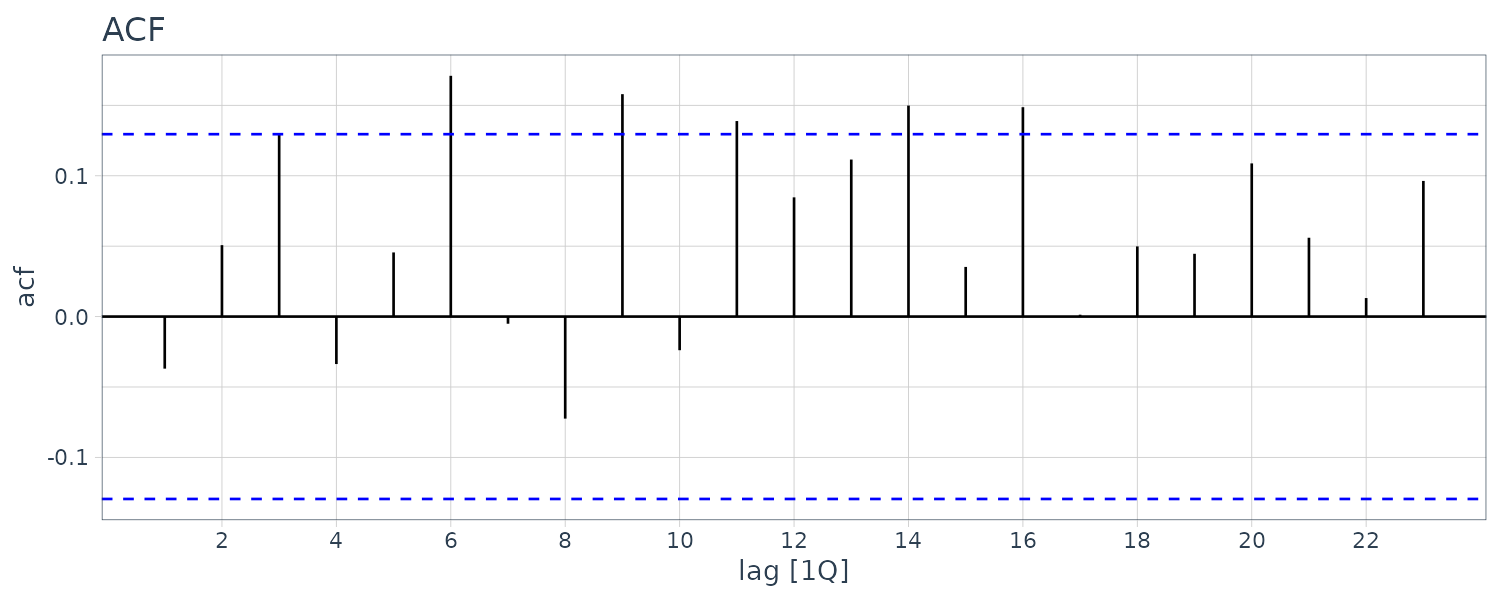
We can see that the residuals are pretty much white noise. This shows that \(e_{t}\) follows a AR(1) process.
The fitted model:
\[\begin{aligned} \hat{\Delta C_{t}} &= 478.6 + 0.03369 \times \Delta C_{t-1} + 0.09908 \times\Delta Y_{t} \end{aligned}\]The delay multipliers from this model are:
\[\begin{aligned} \beta_{0} &= 0.0991\\ \beta_{1} &= 0.0991 \times 0.3369\\ &= 0.0334\\ \beta_{2} &= 0.0991 \times 0.3369^{2}\\ &= 0.0112\\ &\ \ \vdots\\ \end{aligned}\]And the total multiplier:
\[\begin{aligned} \frac{0.0991}{1 - 0.3369} &= 0.149 \end{aligned}\]\(\beta_{0}\) may seem low for what could be interpreted as a marginal propensity to consume. However, because a trend term is included in the model, we are measuring departures from that trend.
Testing the residuals for autocorrelation via the Ljung test:
> cons_inc |>
  features(
    residuals,
    ljung_box,
    lag = 1
  )
# A tibble: 1 × 2
  lb_stat lb_pvalue
    <dbl>     <dbl>
1   0.314     0.575
This shows that \(v_{t}\) is not autocorrelated and hence imply that \(e_{t}\) follows an AR(1) model.
Deriving Multipliers from an ARDL Representation
Instead of beginning with the IDL representation and choosing restrictions a priori, an alternative strategy is to begin with an ARDL representation whose lags have been chosen using conventional model selection criteria and to derive the restrictions on the IDL model implied by the chosen ARDL model.
Suppose we estimate a finite number of \(\theta\) and \(\beta\) from an ARDL model:
\[\begin{aligned} y_{t} &= \delta + \theta_{1}y_{t-1} + \cdots + \theta_{p}y_{t-p} + \delta_{0}x_{t} + \delta_{1}x_{t-1} + \cdots + \delta_{q}x_{t-q} + v_{t} \end{aligned}\]The strategy is to find \(\beta\)’s in the IDL model such that:
\[\begin{aligned} y_{t} &= \alpha + \beta_{0}x_{t} + \beta_{1}x_{t-1} + \cdots + e_{t} \end{aligned}\]Rewriting the ARDL model in terms of lag operators:
\[\begin{aligned} y_{t} &= \delta + \theta_{1}Ly_{t} + \cdots + \theta_{p}L_{p}y_{t} + \delta_{0}x_{t} + \delta_{1}Lx_{t} + \cdots + \delta_{q}L^{q}x_{t} + v_{t} \end{aligned}\]Then we can express:
\[\begin{aligned} (1 - \theta_{1}L - \theta_{2}L^{2} - \cdots - \theta_{p}L^{p})y_{t} &= \delta + (\delta_{0} + \delta_{1}L + \cdots + \delta_{q}L^{q})x_{t} + v_{t} \end{aligned}\]Example: Deriving Multipliers for an Infinite Lag Okun’s Law Model
Recall the earlier Okun’s Law example where we estimated a finite distributed lag model to 4 lags of GDP growth. The coefficient for \(G_{t-1}\) is greater than \(G_{t}\) which suggest a geometrically declining lag would not be appropriate. After experimenting with different values for p and q, we settled on a ARDL(2, 1) model:
\[\begin{aligned} \Delta U_{t} &= \delta + \theta_{1}\Delta U_{t-1} + \theta_{2}\Delta U_{t-1} + \delta_{0}G_{t} + \delta_{1}G_{t-1} + v_{t} \end{aligned}\]Rewriting in lag operator:
\[\begin{aligned} (1 - \theta_{1}L - \theta_{2}L^{2})\Delta U_{t} &= \delta + (\delta_{0} + \delta_{1}L)G_{t} + v_{t} \end{aligned}\]Multiplying both sides by the inverse, we could write:
\[\begin{aligned} \Delta U_{t} &= \frac{\delta}{1 - \theta_{1}L - \theta_{2}L^{2}} + \frac{(\delta_{0} + \delta_{1}L)}{1 - \theta_{1}L - \theta_{2}L^{2}}G_{t} + \frac{v_{t}}{1 - \theta_{1}L - \theta_{2}L^{2}} \end{aligned}\]We could equate that with the IDL representation:
\[\begin{aligned} \Delta U_{t} &= \alpha + \beta_{0}G_{t} + \beta_{1}G_{t-1} + \cdots + e_{t}\\ &= \alpha + (\beta_{0} + \beta_{1}L + \beta_{2}L^{2} + \cdots)G_{t} + e_{t} \end{aligned}\]For them to be identical:
\[\begin{aligned} \alpha &= \frac{\delta}{1 - \theta_{1}L - \theta_{2}L^{2}} \end{aligned}\] \[\begin{aligned} \beta_{0} + \beta_{1}L + \beta_{2}L^{2} + \cdots &= \frac{\delta_{0} + \delta_{1}L}{1 - \theta_{1}L - \theta_{2}L^{2}} \end{aligned}\] \[\begin{aligned} (\beta_{0} + \beta_{1}L + \beta_{2}L^{2} + \cdots)(1 - \theta_{1}L - \theta_{2}L^{2}) &= \delta_{0} + \delta_{1}L\\ \beta_{0} - \beta_{0}\theta_{1}L - \beta_{0}\theta_{2}L^{2} + \beta_{1}L - \theta_{1}\beta_{1}L^{2} - \beta_{1}\theta_{2}L^{3} + \beta_{2}L^{2} - \cdots &= \delta_{0} + \delta_{1}L \end{aligned}\] \[\begin{aligned} e_{t} &= \frac{v_{t}}{1 - \theta_{1}L - \theta_{2}L^{2}} \end{aligned}\]Matching coefficients of like powers yields:
\[\begin{aligned} \alpha &= \frac{\delta}{1 - \theta_{1} - \theta_{2}}\\ \delta_{0} &= \beta_{0}\\ \delta_{1} &= \beta_{1} - \theta_{1}\beta_{0}\\ 0 &= \beta_{2} - \theta_{1}\beta_{1}- \theta_{2}\beta_{0}\\ 0 &= \beta_{3} - \theta_{1}\beta_{2}- \theta_{2}\beta_{1}\\ &\ \ \vdots\\ \beta_{j} &= \theta_{1}\beta_{j-1} + \theta_{2}\beta_{j-2}\\ \end{aligned}\] \[\begin{aligned} j &\geq 2 \end{aligned}\]In general it is easier to just multiply out the expression and equate coefficients of like powers in the lag operator:
\[\begin{aligned} \delta_{0} + \delta_{1}L + \delta_{2}L^{2} + \cdots + \delta_{q}L^{1} = &\ (1 - \theta_{1}L - \theta_{2}L^{2} - \cdots - \theta_{p}L^{p})\ \times\\ &\ (\beta_{0} + \beta_{1}L + \beta_{2}L^{2} + \beta_{3}L^{3} + \cdots) \end{aligned}\]Example: Computing the Multiplier Estimates for the Infinite Lag Okun’s Law Model
Let’s fit the ARDL(2, 1) in R:
fit <- lm(
  du ~ lag(du) +
    lag(du, 2) +
    g +
    lag(g),
  data = okun5_aus
)

> summary(fit)
Call:
lm(formula = du ~ lag(du) + lag(du, 2) + g + lag(g),
   data = okun5_aus)

Residuals:
     Min       1Q   Median       3Q      Max
-0.70307 -0.13774 -0.00876  0.14166  1.07895

Coefficients:
            Estimate Std. Error t value Pr(>|t|)
(Intercept)  0.17079    0.03281   5.206 6.49e-07 ***
lag(du)      0.26395    0.07669   3.442 0.000755 ***
lag(du, 2)   0.20724    0.07200   2.878 0.004605 **
g           -0.09040    0.02442  -3.703 0.000303 ***
lag(g)      -0.12965    0.02523  -5.140 8.75e-07 ***
---
Signif. codes:  0 ‘***’ 0.001 ‘**’ 0.01 ‘*’ 0.05 ‘.’ 0.1 ‘ ’ 1

Residual standard error: 0.2225 on 145 degrees of freedom
  (3 observations deleted due to missingness)
Multiple R-squared:  0.5033,	Adjusted R-squared:  0.4896
F-statistic: 36.73 on 4 and 145 DF,  p-value: < 2.2e-16
Using the relationships we derived earlier, the impact mutliplier and delay multipliers for the first 4 quarters:
\[\begin{aligned} \hat{\beta}_{0} &= \hat{\delta}_{0}\\ &= -0.0904 \end{aligned}\] \[\begin{aligned} \hat{\beta}_{1} &= \hat{\delta}_{1} + \hat{\theta}_{1}\hat{\beta}_{0}\\ &= -0.129647 - 0.263947 \times 0.090400\\ &= -0.1535\\ \hat{\beta}_{2} &= \hat{\theta}_{1}\hat{\beta}_{1} + \hat{\theta}_{2}\hat{\beta}_{0}\\ &= -0.263947 \times 0.153508 - 0.207237 \times 0.0904\\ &= -0.0593 \end{aligned}\] \[\begin{aligned} \hat{\beta}_{3} &= \hat{\theta}_{1}\hat{\beta}_{2} + \hat{\theta}_{2}\hat{\beta}_{1}\\ &= -0.0475\\ \hat{\beta}_{4} &= \hat{\theta}_{1}\hat{\beta}_{3} + \hat{\theta}_{2}\hat{\beta}_{2}\\ &= -0.0248 \end{aligned}\]An increase in GDP growth leads to a fall in unemployment. The effect increases from the current quarter to the next quarter, declines dramatically after that and then gradually declines to zero.
To get the total mulitiplier, we look at the long-run equilibrium by stripping out the time component:
\[\begin{aligned} \Delta U &= 0.1708 + 0.2639\Delta U + 0.2072\Delta U - 0.0904G - 0.1296 G\\ &= \frac{0.1708 − (0.0904 + 0.1296)G}{1 − 0.2639 − 0.2072}\\ &= 0.3229 - 0.4160G \end{aligned}\]The total multiplier can be calculated by taking the derivative:
\[\begin{aligned} \frac{d(\Delta U)}{dG} &= -0.416 \end{aligned}\]We can verify this by summing up the first 10 multipliers:
\[\begin{aligned} \sum_{s=0}^{10}\hat{\beta}_{s} &= -0.414 \end{aligned}\]Finally, the estimate of the normal growth rate that is needed to maintain a constant rate of unemployment is:
\[\begin{aligned} \hat{G}_{N} &= \frac{-\hat{\alpha}}{\sum_{j=0}^{\infty}\hat{\beta}_{j}}\\[5pt] &= \frac{0.3229}{0.416}\\[5pt] &= 0.78% \end{aligned}\]In order to use the least squares to estimate the ARDL model we need to see whether the error term will be such that the estimator is consistent:
\[\begin{aligned} e_{t} &= \frac{v_{t}}{1 - \theta_{1}L - \theta_{2}L^{2}} \end{aligned}\] \[\begin{aligned} (1 - \theta_{1}L - \theta_{2}L^{2})e_{t} &= v_{t}\\ e_{t} - \theta_{1}e_{t-1} - \theta_{2}e_{t-2} &= v_{t} \end{aligned}\] \[\begin{aligned} e_{t} &=\theta_{1}e_{t-1} + \theta_{2}e_{t-2} + v_{t} \end{aligned}\]In general, for \(v_{t}\) to be uncorrelated, the errors for the general ARDL(p, q) model must follow an AR(p) process:
\[\begin{aligned} e_{t}&= \theta_{1}e_{t-1} + \theta_{2}e_{t-2} + \cdots + \theta_{p}e_{t-p} + v_{t} \end{aligned}\]Example: Testing for Consistency of Least Squares Estimation of Okun’s Law
The assumption is that the errors in the IDL representation follow an AR(2) process:
\[\begin{aligned} e_{t} &= \rho_{1}e_{t-1} + \rho_{2}e_{t-2} + v_{t} \end{aligned}\]Given the ARDL representation:
\[\begin{aligned} \Delta U_{t} &= \delta + \theta_{1}\Delta U_{t-1} + \theta_{2}\Delta U_{t-1} + \delta_{0}G_{t} + \delta_{1}G_{t-1} + v_{t} \end{aligned}\]The hypotheses are:
\[\begin{aligned} H_{0}:\ &\rho_{1} &= \theta_{1}, \rho_{2} = \theta_{2}\\ H_{1}:\ & \rho_{1} &\neq \theta_{1}, \rho_{2} \neq \theta_{2} \end{aligned}\]Retrieving \(R^{2}\) in R:
num_zeros <- 3
okun5_aus$e <- 0
theta1 <- as.numeric(coef(fit)[2])
theta2 <- as.numeric(coef(fit)[3])
for (i in (num_zeros + 1):nrow(okun5_aus)) {
  okun5_aus$e[i] <- theta1 * errs[i - 1] +
    theta2 * errs[i - 2] +
    as.numeric(okun5_aus$residuals[i])
}

fit2 <- lm(
  residuals ~ lag(u) + lag(u, 2) +
    g + lag(g) +
    lag(e) + lag(e, 2),
  data = okun5_aus
)

> summary(fit2)$r.squared
[1] 0.02991428
The test-statistic:
\[\begin{aligned} \chi^{2} &= (T - 3) \times R^{2}\\ &= 150 \times 0.02991\\ &= 4.4865 \end{aligned}\]The 5% critical value is:
> qchisq(0.95, 2)
[1] 5.991465Hence, we fail to reject \(H_{0}\) at a 5% significance level. There is not sufficient evidence to conclude that serially correlated errors are a source of inconsistency.
Assumptions for the Infinite Distributed Lag Model
Assumption 1
The time series \(y, x\) are stationary and weakly dependent.
Assumption 2
The corresponding ARDL(p, q) model is:
\[\begin{aligned} y_{t} &= \delta + \theta_{1}y_{t-1} + \cdots + \theta_{p}y_{t-p} + \delta_{0}x_{t}+ \delta_{1}x_{t-1} + \cdots + \delta_{q}x_{t-q} + v_{t} \end{aligned}\] \[\begin{aligned} v_{t} &= e_{t} - \theta_{1}e_{t-1} + \cdots - \theta_{p}e_{t-p} \end{aligned}\]Assumption 3
The errors \(e_{t}\) are strictly exogenous:
\[\begin{aligned} E[e_{t}\mid \textbf{X}] &= 0 \end{aligned}\]Where \(\textbf{X}\) includes all current, past, and future values of \(x\).
Assumption 4
The errors \(e_{t}\) follow the AR(p) process:
\[\begin{aligned} e_{t}&= \theta_{1}e_{t-1} + \theta_{2}e_{t-2} + \cdots + \theta_{p}e_{t-p} + u_{t} \end{aligned}\]Where \(u_{t}\) is exogenous with respect to current and past values of \(x\) and past values of \(y\):
\[\begin{aligned} E[u_{t}\mid x_{t}, x_{t-1}, y_{t-1}, x_{t-2}, y_{t-2}, \cdots] = 0 \end{aligned}\]And homoskedastic:
\[\begin{aligned} \textrm{var}(u_{t}\mid x_{t}) &= \sigma_{u}^{2} \end{aligned}\]Alternative Assumption 5
And alternative assumption to this is that the errors \(e_{t}\) are uncorrelated, and:
\[\begin{aligned} \text{cov}(e_{t}, e_{s}\mid x_{t}, x_{s}) &= 0\\ t &\neq s\\ \text{var}(e_{t}\mid x_{t}) &= \sigma_{e}^{2} \end{aligned}\]In this case, the errors follow an MA(p)process
\[\begin{aligned} v_{t} &= e_{t} - \theta_{1}e_{t-1}- \theta_{2}e_{t-2}- \cdots - \theta_{p}e_{t-p} \end{aligned}\]But the least squares will be inconsistent and the instrumental variables approach can be used as an alternative.
Finally, we note that both an FDL model with autocorrelated errors and an IDL model can be transformed to ARDL models. Thus, an issue that arises after estimating an ARDL model is whether to interpret it as an FDL model with autocorrelated errors or an IDL model.
An attractive way out of this dilemma is to assume an FDL model and use HAC standard errors. In many cases, an IDL model will be well approximated by an FDL, and using HAC standard errors avoids having to make the restrictive strict exogeneity assumption.
Nonstationarity
An important assumption that we have assumed so far is that the variables are stationary and weakly dependent. That means the time-series have means and variances that do not change over time, and autocorrelations that depend only on the time between observations. Furthermore, the autocorrelations die out as the distance between observations increases. However, many economic time series are not stationary. Their means and/or variances change over time, and their autocorrelations do not die out or they decline very slowly.
Example: Plots of Some U.S. Economic Time Series
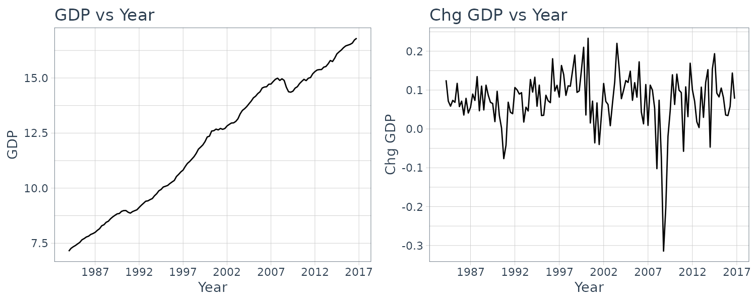
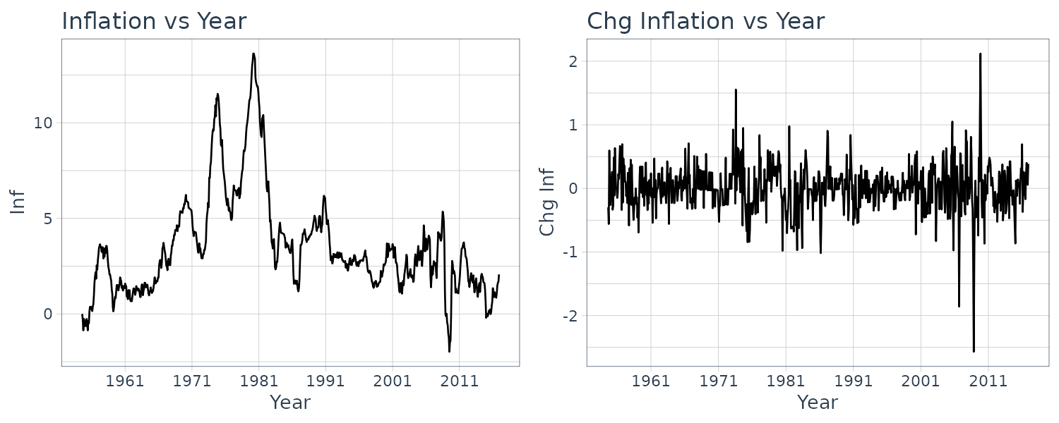
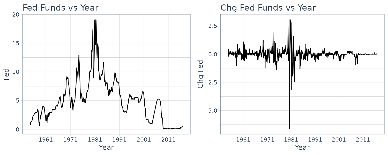
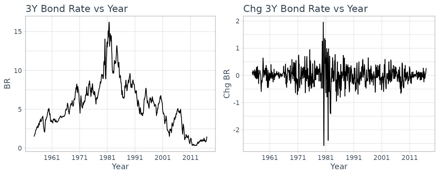
In summary, stationary time series have the following properties:
\[\begin{aligned} E[y_{t}] &= \mu\\ y_{t} &= \sigma^{2}\\ \textrm{cov}(y_{t}, y_{t+s}) &= \textrm{cov}(y_{t}, y_{t-s})\\ &= \gamma_{s} \end{aligned}\]Having a constant mean and variations in the series that tend to return to the mean are characteristics of stationary variables. They have the property of mean reversion. Furthermore, stationary weakly dependent series have autocorrelations that cut off or tend to decline geometrically and dying out at long lags. Whereas nonstationary time-series have autocorrelations that die out linearly.
Trend Stationary Variables
Trends can be categorized as a stochastic trend or a deterministic trend, and sometimes both. Variables that are stationary after “subtracting out”” a deterministic trend are called trend stationary.
The simplest model for a deterministic trend for a variable \(y\) is the linear trend model:
\[\begin{aligned} y_{t} &= c_{1} + c_{2}t + u_{t} \end{aligned}\]The coefficient \(c_{2}\) gives the change in \(y\) from a period to the next assuming \(\Delta u_{t} = 0\):
\[\begin{aligned} y_{t} - y_{t-1} &= (c_{1} + c_{2}t) - (c_{1} + c_{2}(t - 1)) + \Delta u_{t}\\ &= c_{2} \end{aligned}\]The trend \(c_{1} + c_{2}t\) is called a determinstic trend because it does not contain a stochastic component. \(y_{t}\) is trend stationary if its fluctuations around this trend \(u_{t}\) are stationary:
\[\begin{aligned} u_{t} &= y_{t}- (c_{1} + c_{2}t) \end{aligned}\]When \(y_{t}\) is trend stationary, we can use least squares to find \(\hat{c}_{1}, \hat{c}_{2}\) and remove the trend:
\[\begin{aligned} \hat{u}_{t} &= y_{t} - (\hat{c}_{1} + \hat{c}_{2}t) \end{aligned}\]We simulate an example in R:
c1 <- 0.1
c2 <- 0.05
for (i in 2:n) {
  dat$y[i] <- c1 +
    c2 * i +
    dat$e[i]
}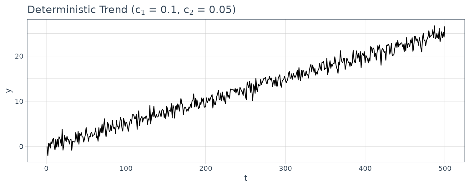
Consider the regression between 2 trend stationary variables. Suppose:
\[\begin{aligned} y_{t} &= c_{1} + c_{2}t + u_{t}\\ x_{t} &= d_{1} + d_{2}t + v_{t} \end{aligned}\]First, we remove the trend via least squares estimates of the coefficients:
\[\begin{aligned} \tilde{y}_{t} &= y_{t} - (\hat{c}_{1} + \hat{c}_{2}t)\\ \tilde{x}_{t} &= x_{t} - (\hat{d}_{1} + \hat{d}_{2}t) \end{aligned}\]A suitable model where changes in \(y\) around the trend are related to changes in \(x\) around its trend is:
\[\begin{aligned} \tilde{y}_{t} &= \beta\tilde{x}_{t} + u_{t} \end{aligned}\]Note that no intercept is required because \(\tilde{y}_{t}, \tilde{x}_{t}\) are OLS residuals with zero means. It can be shown via the FWL theorem that the following equation will give an equivalent estimate for \(\beta\):
\[\begin{aligned} y_{t} &= \alpha_{0} + \alpha_{1}t + \beta x_{t} + u_{t} \end{aligned}\]For more general ARDL models:
\[\begin{aligned} \tilde{y}_{t} &= \sum_{s=1}^{p}\theta_{s}\tilde{y}_{t-s} + \sum_{r=0}^{q}\delta_{r}\tilde{x}_{t-r} + u_{t} \end{aligned}\] \[\begin{aligned} y_{t} &= \alpha_{0} + \alpha_{1}t + \sum_{s=1}^{p}\theta y_{t-s} + \sum_{r = 0}^{q}\delta_{r}x_{t-r} + u_{t} \end{aligned}\]We have discovered that regression relationships between trend stationary variables can be modeled by removing the deterministic trend from the variables, making them stationary, or by including the deterministic trend directly in the equation. However, we have not shown how to distinguish between deterministic and stochastic trend.
Other Trends
Another popular trend is when the variable grows at a percentage rate \(a_{2}\):
\[\begin{aligned} y_{t} &= y_{t-1} + a_{2}y_{t-1} \end{aligned}\] \[\begin{aligned} \frac{y_{t} - y_{t-1}}{y_{t-1}} &= a_{2} 100 \times \frac{y_{t} - y_{t-1}}{y_{t-1}} &= 100 a_{2}\% \end{aligned}\]Recall that relative change can be approximated by:
\[\begin{aligned} \frac{y_{t} - y_{t-1}}{y_{t-1}} &\approx \Delta \ln(y_{t})\\ &= \ln(y_{t}) - \ln(y_{t-1})\\ &\approx \%\Delta y_{t}\\ &= 100 a_{2} \end{aligned}\]A model with this property would thus be:
\[\begin{aligned} \ln(y_{t}) &= a_{1} + a_{2}t + u_{t} \end{aligned}\]This is because:
\[\begin{aligned} E[\ln(y_{t}) - \ln(y_{t}-1)] &= a_{1} + a_{2}t - a_{1} - a_{2}(t-1)\\ &= a_{2}(t - (t- 1)) + 0\\ &= a_{2} \end{aligned}\]This would result in a determinstic trend for:
\[\begin{aligned} y_{t} &= e^{a_{1} + a_{2}t} \end{aligned}\]And \(\ln(y_{t})\) would be trend stationary if \(u_{t}\) is stationary.
Other popular trends are polynomial trends such as the cubic trend:
\[\begin{aligned} y_{t} &= \beta_{1} + \beta_{2}t^{3} + e_{t} \end{aligned}\]However most deterministic trends only work well if it is continously increasing or decreasing.
Example: A Deterministic Trend for Wheat Yield
Food production tend to keep pace with a growing population due to science developing new varieties of wheat to increase yield. Hence we expect wheat yield to trend upward over time. But the yield also depends heavily on rainfall which is uncertain. Thus, we expect yield to fuctuate around an increasing trend.
Plotting ln(Yield) and rainfall:
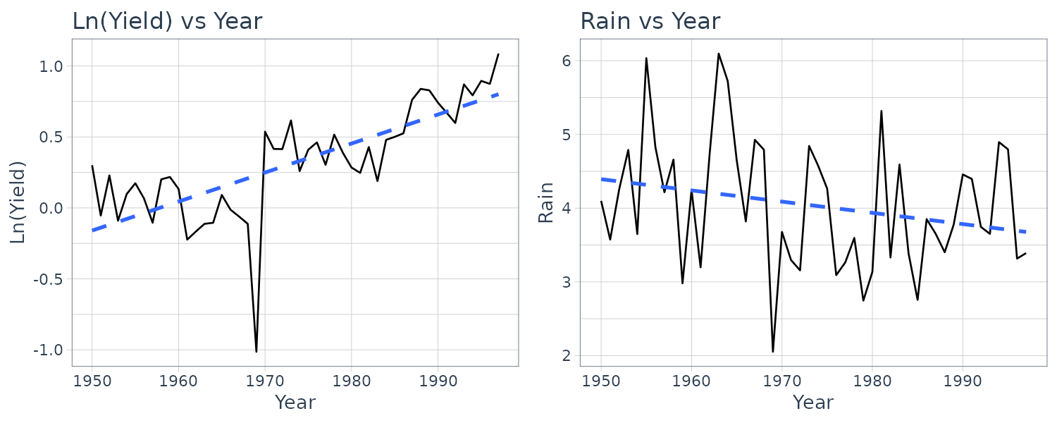
We will add a quadratic term to rainfall as there are signs of decreasing returns to rainfall:
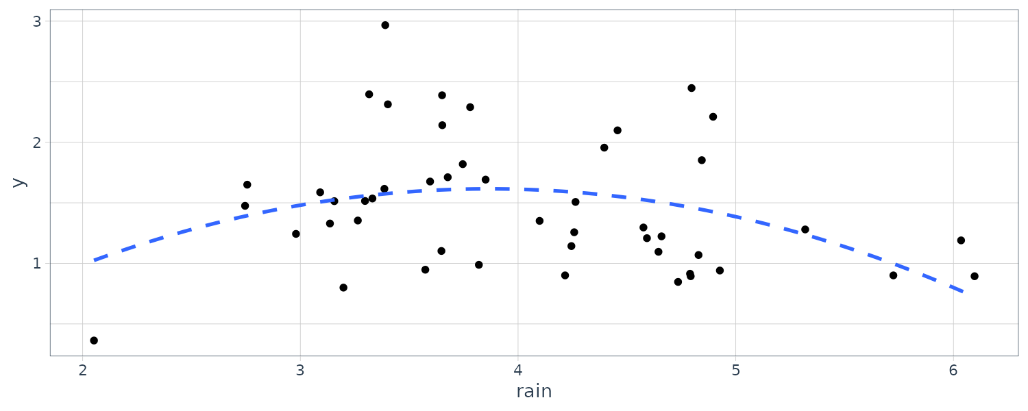
fit <- lm(
  log(y) ~ t +
    rain +
    I(rain^2),
  data = toody5
)

> summary(fit)
Call:
lm(formula = log(y) ~ t + rain + I(rain^2), data = toody5)

Residuals:
     Min       1Q   Median       3Q      Max
-0.68949 -0.13172  0.01845  0.15776  0.52619

Coefficients:
             Estimate Std. Error t value       Pr(>|t|)
(Intercept) -2.510073   0.594383  -4.223       0.000119 ***
t            0.019708   0.002519   7.822 0.000000000727 ***
rain         1.148950   0.290356   3.957       0.000273 ***
I(rain^2)   -0.134388   0.034610  -3.883       0.000343 ***
---
Signif. codes:  0 ‘***’ 0.001 ‘**’ 0.01 ‘*’ 0.05 ‘.’ 0.1 ‘ ’ 1

Residual standard error: 0.2326 on 44 degrees of freedom
Multiple R-squared:  0.6637,	Adjusted R-squared:  0.6408
F-statistic: 28.94 on 3 and 44 DF,  p-value: 0.0000000001717
Assuming the outcome and predictors are all trend stationary, we can replicate the same thing by detrending each variable:
fit_y <- lm(log(y) ~ t, data = toody5)
fit_rain <- lm(rain ~ t, data = toody5)
fit_rain2 <- lm(I(rain^2) ~ t, data = toody5)

toody5 <- toody5 |>
  mutate(
    ry = log(y) - fit_y$fitted.values,
    rrain = rain - fit_rain$fitted.values,
    rrain2 = rain^2 - fit_rain2$fitted.values
  )

fit <- lm(
  ry ~ rrain + rrain2,
  data = toody5
)

> summary(fit)
Call:
lm(formula = ry ~ rrain + rrain2, data = toody5)

Residuals:
     Min       1Q   Median       3Q      Max
-0.68949 -0.13172  0.01845  0.15776  0.52619

Coefficients:
              Estimate Std. Error t value Pr(>|t|)
(Intercept) -4.126e-17  3.320e-02   0.000 1.000000
rrain        1.149e+00  2.871e-01   4.002 0.000232 ***
rrain2      -1.344e-01  3.422e-02  -3.927 0.000293 ***
---
Signif. codes:  0 ‘***’ 0.001 ‘**’ 0.01 ‘*’ 0.05 ‘.’ 0.1 ‘ ’ 1

Residual standard error: 0.23 on 45 degrees of freedom
Multiple R-squared:  0.2633,	Adjusted R-squared:  0.2306
F-statistic: 8.042 on 2 and 45 DF,  p-value: 0.001032
Notice the coefficients to rain and rain quadratic terms are the same.
First-Order Autoregressive Model
The econometric model generating a time series \(y_{t}\) is called a stochastic process. Univariate time-series models (no explanatory variables) are examples of stochastic proceses where a single variable \(y\) is related to past values of itself or/and past error terms.
We first consider an AR(1) model with 0 mean:
\[\begin{aligned} y_{t} &= \rho y_{t-1} + v_{t} \end{aligned}\] \[\begin{aligned} |\rho| &< 1 \end{aligned}\]An example of an AR(1) model with 0 mean:
n <- 500
dat <- tsibble(
  t = 1:n,
  e = rnorm(n),
  y = 0,
  index = t
)

rho <- 0.7
for (i in 2:n) {
  dat$y[i] <- rho * dat$y[i-1] +
    dat$e[i]
}

dat |>
  autoplot(y) +
  xlab("t") +
  ggtitle(latex2exp::TeX("AR(1) $\\rho$ = 0.7")) +
  theme_tq()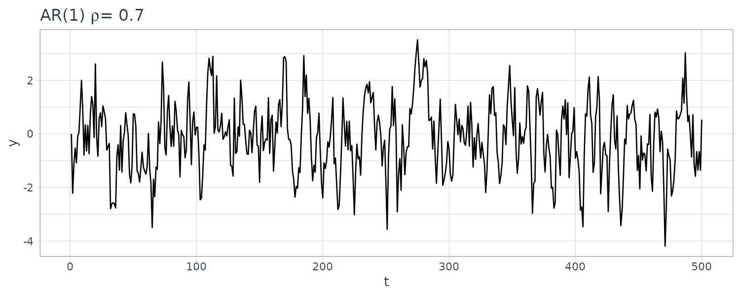
In the context of time-series models, the errors are sometimes known as innovations. The assumption \(\mid \rho \mid < 1\) implies that \(y_{t}\) is stationary.
In general, an AR(p) model includes lags up to \(y_{t-p}\).
Using recursive substitution:
\[\begin{aligned} y_{1} &= \rho y_{0} + v_{1}\\ y_{2} &= \rho y_{1} + v_{2}\\ &= \rho(\rho y_{0} + v_{1}) + v_{2}\\ &= \rho^{2}y_{0} + \rho v_{1} + v_{2}\\ &\ \ \vdots\\ y_{t} &= v_{t} + \rho v_{t-1} + \rho^{2} v_{t-2} + \cdots + \rho^{t}y_{0} \end{aligned}\]The mean of \(y_{t}\):
\[\begin{aligned} E[y_{t}] &= E[v_{t} + \rho v_{t-1} + \rho^{2} v_{t-2} + \cdots + \rho^{t}y_{0}]\\ &= 0 \end{aligned}\]The variance of \(y_{t}\):
\[\begin{aligned} \text{var}(y_{t}) &= \text{var}(v_{t}) + \rho^{2}\text{var}(v_{t-1}) + \rho^{4}\text{var}(v_{t-2}) + \rho^{6}\text{var}(v_{t-3})\cdots\\ &= \sigma_{v}^{2} + \rho^{2}\sigma_{v}^{2} + \rho^{4}\sigma_{v}^{2} + \rho^{6}\sigma_{v}^{2}\cdots\\ &= \sigma_{v}^{2}(1 + \rho^{2} + \rho^{4} + \rho^{6} + \cdots)\\ &= \frac{\sigma_{v}^{2}}{1 - \rho^{2}} \end{aligned}\]Because the \(v\)’s are uncorrelated, the covariance terms are zero.
And the covariance:
\[\begin{aligned} \text{cov}(y_{t}, y_{t-1}) &= E[y_{t}y_{t-1}]\\ &= E[(v_{t} + \rho v_{t-1} + \rho^{2}v_{t-2} + \cdots)(v_{t-1} + \rho v_{t-2} + \rho^{2}v_{t-3} + \cdots)]\\ &= \rho E[v_{t-1}^{2}] + \rho^{3}E[v_{t-2}^{2}] + \rho^{5}E[v_{t-3}^{2} + \cdots]\\ &= \rho\sigma_{v}^{2}(1 + \rho^{2} + \rho^{4} + \cdots)\\ &= \frac{\rho \sigma_{v}^{2}}{1 - \rho^{2}} \end{aligned}\]We can show that the covariance that are s periods apart is:
\[\begin{aligned} \text{cov}(y_{t}, y_{t-s}) &= \frac{\rho^{s} \sigma_{v}^{2}}{1 - \rho^{2}} \end{aligned}\]Incorporating a mean of \(\mu\) for \(y_{t}\):
\[\begin{aligned} (y_{t} - \mu) &= \rho(y_{t-1} - \mu) + v_{t}\\ y_{t} &= \mu(1 - \rho) + \rho y_{t-1} + v_{t}\\ y_{t} &= \alpha + \rho y_{t-1} + v_{t} \end{aligned}\] \[\begin{aligned} \alpha &= \mu(1 - \rho) \end{aligned}\] \[\begin{aligned} |\rho| &< 1 \end{aligned}\]We can either work with the de-meaned variable \((y_{t} - \mu)\) or introduce the intercept term \(\alpha\).
Another extension is to consider an AR(1) model fluctuating around a linear trend:
\[\begin{aligned} \mu + \delta t \end{aligned}\]In this case, the detrended series \((y_{t} - \mu - \delta t)\) behave like an AR(1) model:
\[\begin{aligned} (y_{t} - \mu - \delta t) &= \rho(y_{t} - \mu - \delta t) + v_{t} \end{aligned}\] \[\begin{aligned} |\rho| < 1 \end{aligned}\]Which can be rearranged as:
\[\begin{aligned} y_{t} &= \alpha + \rho y_{t-1} + \lambda t + v_{t} \end{aligned}\] \[\begin{aligned} \alpha &= \mu(1 - \rho) + \rho\delta\\ \lambda &= \delta(1 - \rho) \end{aligned}\] \[\begin{aligned} |\rho| &< 1 \end{aligned}\]An example in R:
rho <- 0.7
alpha <- 1
lambda <- 0.01

for (i in 2:n) {
  dat$y[i] <- alpha +
    rho * dat$y[i - 1]  +
    lambda * i +
    dat$e[i]
}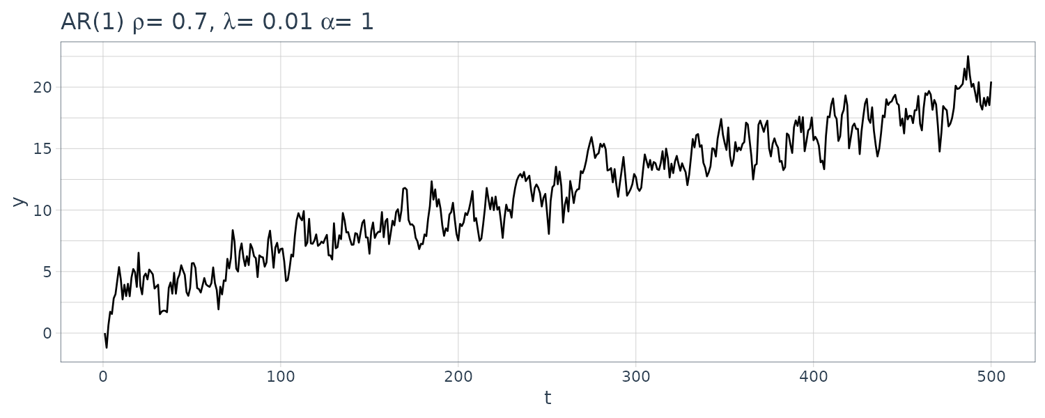
When \(\mid \rho \mid < 1\), the time-series model is an example of a trend-stationary process. The de-trended series has a constant variance, and covariances only depend only on the time separating observations.
Random Walk Models
Consider the case where \(\rho = 1\):
\[\begin{aligned} y_{t} &= y_{t-1} + v_{t} \end{aligned}\]It is called random walk because the series appear to wander upward or downward with no real pattern.
Using recursive substitution:
\[\begin{aligned} y_{1} &= y_{0} + v_{1}\\ y_{2} &= y_{1} + v_{2}\\ &= (y_{0} + v_{1}) + v_{2}\\ &= y_{0} + \sum_{s=1}^{2}v_{s}\\ &\ \ \vdots\\ y_{t} &= y_{t-1} + v_{t}\\ &= y_{0} + \sum_{s=1}^{t}v_{s} \end{aligned}\]\(\sum_{s=1}^{t}v_{s}\) is known as the stochastic trend vs the determinstic trend \(\delta t\). If \(y_{t}\) is subjected to a sequence of positive shocks, followed by a sequence of negative shocks, it will have the appearance of wandering upwards then downwards.
\[\begin{aligned} E[y_{t}] &= y_{0} + \sum_{s = 1}^{t}E[v_{s}]\\ &= y_{0}\\ \mathrm{var}(y_{t}) &= \mathrm{var}\Big(\sum_{s = 1}^{t}v_{s}\Big)\\ &= t\sigma_{v}^{2} \end{aligned}\]We will simulate an example in R:
for (i in 2:n) {
  dat$y[i] <- dat$y[i-1] +
    dat$e[i]
}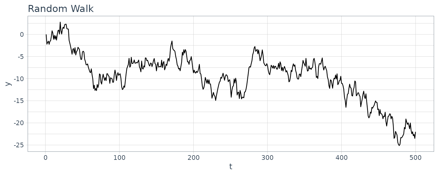
We could also add a drift:
\[\begin{aligned} y_{t} &= \delta + y_{t-1} + v_{t}\\ y_{1} &= \delta + y_{0} + v_{1}\\ y_{2} &= \delta + y_{1} + v_{2}\\ &= \delta + (\delta + y_{0} + v_{1}) + v_{2}\\ &= 2\delta + y_{0} + \sum_{s=1}^{2}v_{s}\\ &\ \ \vdots\\ y_{t} &= \delta + y_{t-1} + v_{t}\\ &= t\delta + y_{0} + \sum_{s=1}^{t}v_{s} \end{aligned}\]The value of y at time t is made up of an initial value \(y_{0}\) , the stochastic trend component \(\sum_{s=1}^{t}v_{s}\) and now a deterministic trend component \(t\delta\). The mean and variance of \(y_{t}\) are:
\[\begin{aligned} E[y_{t}] &= t\delta + y_{0} + \sum_{s = 1}^{t}E[v_{s}]\\ &= t\delta + y_{0}\\ \mathrm{var}(y_{t}) &= \mathrm{var}(\sum_{s = 1}^{t})\\ &= t\sigma_{v}^{2} \end{aligned}\]Let’s simulate an example in R:
drift <- 0.1
for (i in 2:n) {
  dat$y[i] <- drift +
    dat$y[i - 1] +
    dat$e[i]
}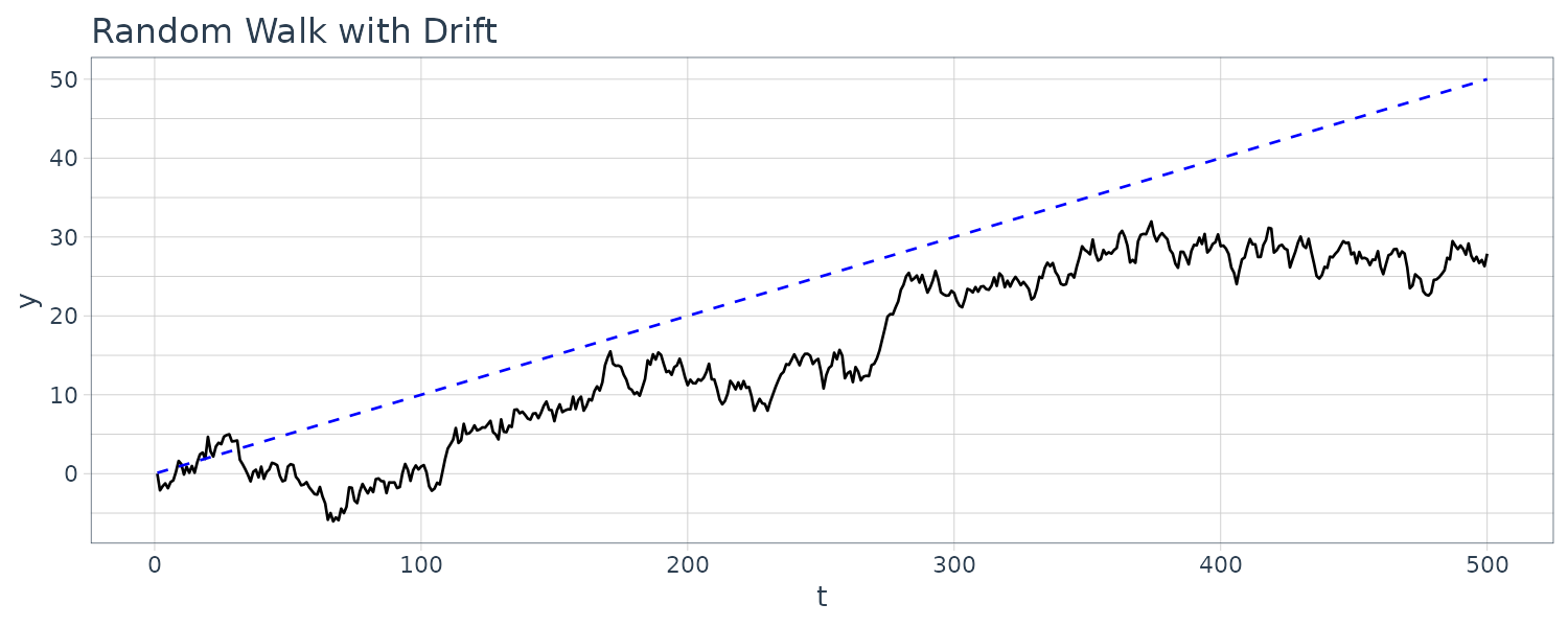
We can extend the random walk model even further by adding a time trend:
\[\begin{aligned} y_{t} &= \alpha + \delta t + y_{t-1} + v_{t}\\ y_{1} &= \alpha + \delta + y_{0} + v_{1}\\ y_{2} &= \alpha + \delta 2 + y_{1} + v_{2}\\ &= \alpha + 2\delta + (\alpha + \delta + y_{0} + v_{1}) + v_{2}\\ &= 2\alpha + 3\delta + y_{0} + \sum_{s=1}^{2}v_{s}\\ &\ \ \vdots\\ y_{t} &= \alpha + \delta t + y_{t-1} + v_{t}\\ &= t\alpha + \frac{t(t+1)}{2}\delta + y_{0} + \sum_{s=1}^{t}v_{s} \end{aligned}\]We have used the sum of an arithmetic progression:
\[\begin{aligned} 1 + 2 + 3 + \cdots + t &= \frac{t(t+1)}{2} \end{aligned}\]Doing an example in R:
alpha <- 0.1
delta <- 0.01
for (i in 2:n) {
  dat$y[i] <- alpha +
    delta * i +
    dat$y[i - 1] +
    dat$e[i]
}
Consequences of Stochastic Trends
We noted that regressions involving variables with a deterministic trend, and no stochastic trend, did not present any difficulties providing the trend was included in the regression relationship, or the variables were detrended. Allowing for the trend was important because excluding it could lead to omitted variable bias. So hereforth, when we refer to nonstationary variables, we generally mean variables that are neither stationary nor trend stationary.
A consequence of regression involving nonstationary variables with stochastic trends is that OLS estimates no longer have approximate normal distributions in large samples, and interval estimates and hypothesis tests will no longer be valid. Precision of estimation may not be what it seems to be and conclusions about relationships between variables could be wrong. One particular problem is that two totally independent random walks can appear to have a strong linear relationship when none exists. This is known as spurious regressions.
Example: A Regression with Two Random Walks
Using the spurious dataset, we plot the two random walks:
spurious$t <- 1:nrow(spurious)

spurious <- spurious |>
  as_tsibble(index = t)

spurious |>
  autoplot(rw1) +
  ylab("") +
  xlab("") +
  geom_line(aes(y = rw2)) +
  theme_tq()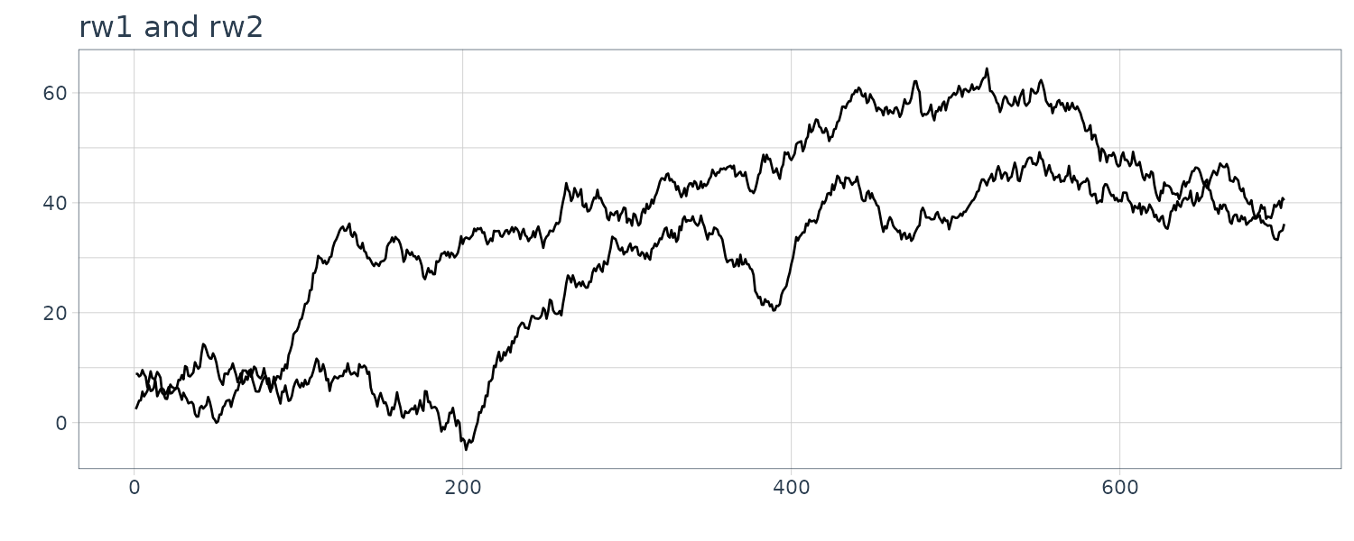
And also the scatterplot:
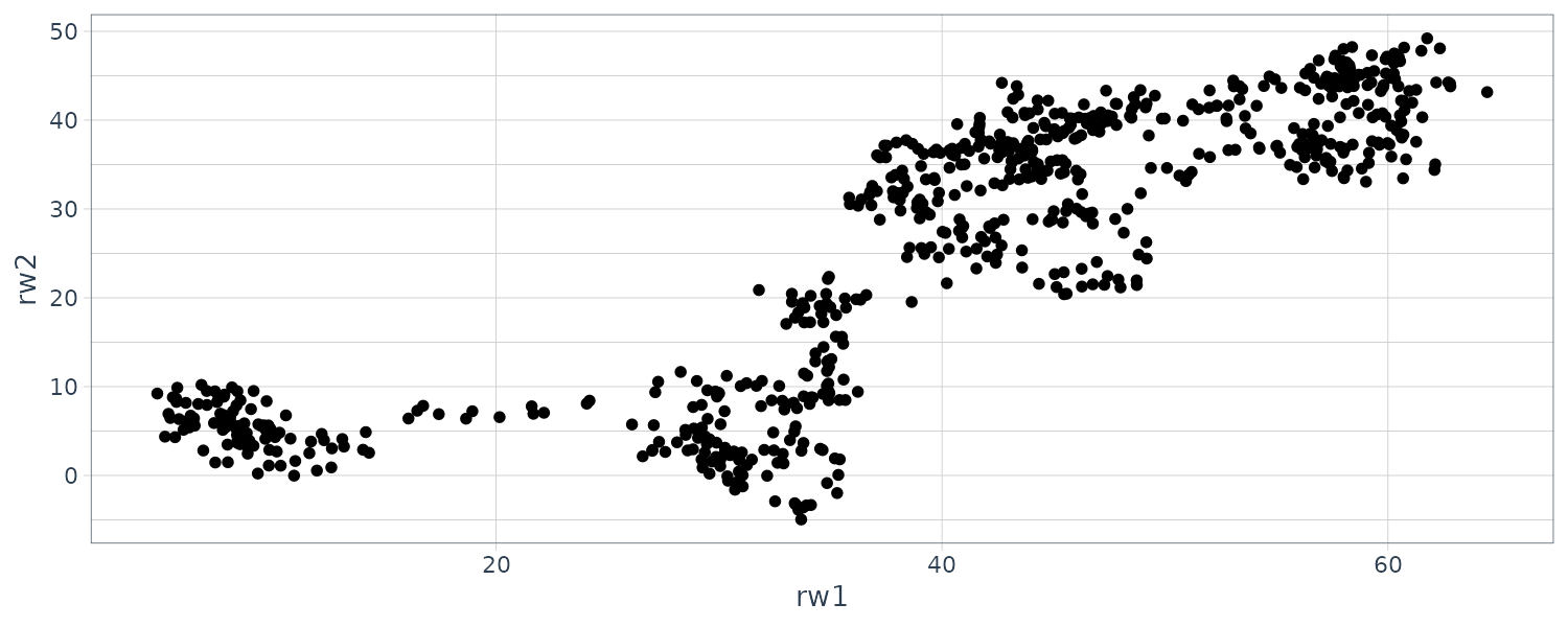
Fitting a regression model:
fit <- lm(
  rw1 ~ rw2,
  data = spurious
)

> summary(fit)
Call:
lm(formula = rw1 ~ rw2, data = spurious)

Residuals:
     Min       1Q   Median       3Q      Max
-20.7746  -6.2759   0.7592   6.7972  20.0396

Coefficients:
            Estimate Std. Error t value Pr(>|t|)
(Intercept) 17.81804    0.62048   28.72   <2e-16 ***
rw2          0.84204    0.02062   40.84   <2e-16 ***
---
Signif. codes:  0 ‘***’ 0.001 ‘**’ 0.01 ‘*’ 0.05 ‘.’ 0.1 ‘ ’ 1

Residual standard error: 8.557 on 698 degrees of freedom
Multiple R-squared:  0.7049,	Adjusted R-squared:  0.7045
F-statistic:  1668 on 1 and 698 DF,  p-value: < 2.2e-16
We can see that the \(R^{2} = 0.7\) is very high. Testing for autocorrelation, we see the result is significant meaning we fail to reject no autocorrelation.
spurious$residuals <- fit$residuals

> spurious |>
  features(residuals, ljung_box, lag = 10)
# A tibble: 1 × 2
  lb_stat lb_pvalue
    <dbl>     <dbl>
1   6085.         0
To summarize, when nonstationary time series are used in a regression model, the results may spuriously indicate a significant relationship when there is none. In these cases the least-squares estimator and least-squares predictor do not have their usual properties, and t-statistics are not reliable. Since many macroeconomic time series are nonstationary, it is particularly important to take care when estimating regressions with macroeconomic variables.
With nonstationary variables each error or shock \(v_{t}\) has a lasting effect, and these shocks accumulate. With stationary variables the effect of a shock eventually dies out and the variable returns to its mean. Whether a change in a macroeconomic variable has a permanent or transitory effect is essential information for policy makers.
Unit Root Tests
Also known as Dickey-Fuller test for a unit root.
For a AR(1) model:
\[\begin{aligned} y_{t} &= \alpha + \rho y_{t-1} + v_{t} \end{aligned}\]\(y_{t}\) is stationary if \(\mid\rho\mid < 1\) and has a unit root if \(\rho=1\).
In general, for a AR(p) model:
\[\begin{aligned} y_{t} &= \alpha + \theta_{1} y_{t-1} + \cdots + \theta_{p}y_{t-p} + v_{t} \end{aligned}\]If the absolute value of the roots of the following polynomial equation is greater than 1, then it is stationary:
\[\begin{aligned} \varphi(z) &= 1 - \theta_{1}z - \cdots - \theta_{p}z^{p} \end{aligned}\] \[\begin{aligned} |z| > 1 \end{aligned}\]When \(p=1\):
\[\begin{aligned} \varphi(z) &= 1 - \theta_{1} z\\ &= 0\\ z &= \frac{1}{\theta_{1}} \end{aligned}\] \[\begin{aligned} |z| &> 1\\ |\theta_{1}| &< 1 \end{aligned}\]For multiple roots, if one of the roots is equal to 1 (rather than greater than 1), then \(y_{t}\) is said to have a unit root and it has a stochastic trend and is nonstationary.
If one of the roots of \(\mid \varphi(z) \mid < 1\), then \(y_{t}\) is non-stationary and explosive. Empirically, we do not observe time series that explode and so we restrict ourselves to unit roots for nonstationarity.
Order of Integration
If a series (such as random walk), can be made stationary by taking the first difference, it is said to be integrated of order one \(I(1)\).
For example, if \(y_{t}\) follows a random walk:
\[\begin{aligned} \delta y_{t} &= y_{t} - y_{t-1}\\ &= v_{t} \end{aligned}\]Stationary series are said to be \(I(0)\). In general, the order of integration of a series is the minimum number of time it is differenced to be stationary.
Example: The Order of Integration of the Two Interest Rate Series
To find their order of integration, we ask the question that whether their first differences are stationary:
\[\begin{aligned} \Delta FFR_{t} &= FFR_{t} - FFR_{t-1}\\ \Delta BR_{t} &= BR_{t} - BR_{t-1} \end{aligned}\]In this example, we will just employ PP test for unit roots. Note that the null hypothesis is that the unit roots is 1 and alternative hypothesis is greater than 1.
> usdata5 |>
  features(
    ffr, unitroot_pp
  )
# A tibble: 1 × 2
  pp_stat pp_pvalue
    <dbl>     <dbl>
1   -2.28       0.1

> usdata5 |>
  features(
    dffr, unitroot_pp
  )
# A tibble: 1 × 2
  pp_stat pp_pvalue
    <dbl>     <dbl>
1   -17.5      0.01

> usdata5 |>
  features(
    br, unitroot_pp
  )
# A tibble: 1 × 2
  pp_stat pp_pvalue
    <dbl>     <dbl>
1   -1.78       0.1

> usdata5 |>
  features(
    dbr, unitroot_pp
  )
# A tibble: 1 × 2
  pp_stat pp_pvalue
    <dbl>     <dbl>
1   -18.4      0.01
As we can see, both series have unit roots and roots greater than 1 after taking a first difference.
Unit Root Tests
Dickey-Fuller
Null hypothesis is that \(y_{t}\) has a unit root and the alternative that \(y_{t}\) is stationary. Note that Dickey-Fuller test has low power. That is they often cannot distinguish between a highly persistent stationary process (where ρ is very close but not equal to 1) and a nonstationary process (where ρ = 1).
Null hypothesis is nonstationary.
Elliot, Rothenberg, and Stock (ERS)
The ERS test proposes removing the constant/trend effects from data and performing unit root test on the residuals.
Null hypothesis is nonstationary.
Philips and Perron (PP)
Adopts a nonparametric approach that assumes a general ARMA structure and uses spectral methods to estimate the standard error of the test correlation.
Null hypothesis is nonstationary.
Kwiatkowski, Phillips, Schmidt, and Shin (KPSS)
KPSS specifies a null hypothesis that the series is stationary or trend stationary rather than DF nonstationary null hypothesis.
Ng and Perron (NP)
Modifications of ERS and PP tests.
Cointegration
In general, we avoid using nonstationary time-series variables in regression models as it tend to give spurious regression. If \(y_{t}, x_{t}\) are nonstationary I(1) variables, we would expect their difference (or any linear combination) to be I(1) as well. However, there is a special case where both \(y_{t}\) and \(x_{t}\) are I(1) nonstationary, but \(e_{t}\) is I(0) stationary:
\[\begin{aligned} e_{t} &= y_{t} - \beta_{0} - \beta_{1}x_{t} \end{aligned}\]A way to test whether \(y_{t}, x_{t}\) are cointegrated is to test whether the errors \(e_{t}\) are stationary. If the residuals are stationary, then \(y_{t}, x_{t}\) are said to be cointegrated. If the residuals are nonstationary, then \(y_{t}, x_{t}\) are not cointegrated, and any apparent regression relationship between them is said to be spurious.
\(y_{t}\) and \(x_{t}\) are said to be cointegrated. It implies that they share similar stochastic trends and their difference is stationary (do not diverge too far from each other).
The test for stationarity of the residuals is based on the test equation:
\[\begin{aligned} \Delta \hat{e}_{t} &= \gamma\hat{e}_{t-1} + v_{t} \end{aligned}\]Example: Are the Federal Funds Rate and Bond Rate Cointegrated?
Fitting the model in R:
fit <- lm(br ~ ffr, data = usdata5)

> summary(fit)
Call:
lm(formula = br ~ ffr, data = usdata5)

Residuals:
    Min      1Q  Median      3Q     Max
-4.1928 -0.5226 -0.1033  0.5762  2.8722

Coefficients:
            Estimate Std. Error t value Pr(>|t|)
(Intercept) 1.327693   0.059275   22.40   <2e-16 ***
ffr         0.832029   0.009707   85.72   <2e-16 ***
---
Signif. codes:  0 ‘***’ 0.001 ‘**’ 0.01 ‘*’ 0.05 ‘.’ 0.1 ‘ ’ 1

Residual standard error: 0.958 on 747 degrees of freedom
Multiple R-squared:  0.9077,	Adjusted R-squared:  0.9076
F-statistic: 7347 on 1 and 747 DF, p-value: < 2.2e-16Checking the ACF:
usdata5$residuals <- fit$residuals

usdata5 |>
  ACF(residuals) |>
  autoplot() +
  ggtitle("ACF") +
  theme_tq()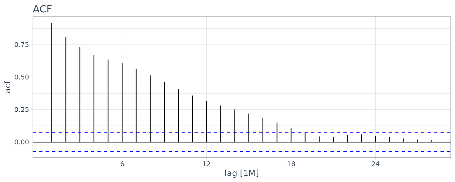
The ACF shows the residuals is not a white noise, but are the residuals nonstationary? Let us check for unit roots:
usdata5 |>
  features(
    residuals,
    unitroot_pp
  )
> # A tibble: 1 × 2
  pp_stat pp_pvalue
    <dbl>     <dbl>
1   -5.62      0.01
We can reject the null hypothesis that the residuals are nonstationary at the 5% significance level.
This shows that federal funds and bond rates are cointegrated. It means that when the Federal Reserve implements monetary policy by changing the federal funds rate, the bond rate will also change thereby ensuring that the effects of monetary policy are transmitted to the rest of the economy.
Error Correction Model
A relationship between I(1) variables is often referred to as a long-run relationship and a relationship between I(0) variables are referred to as a short-run relation. In this section, we describe a dynamic relationship between I(0) variables, which embeds a cointegrating relationship, known as the short-run error correction model.
Let us consider a ARDL model with both \(y, x\) as nonstationary. We start off with lags up to order one, but it holds for any order of lags.
\[\begin{aligned} y_{t} &= \delta + \theta_{1}y_{t-1} + \delta_{0}x_{t} + \delta_{1}x_{t-1} + v_{t} \end{aligned}\]If \(y, x\) are cointegrated, it means that there is a long-run relationship between them. To derive this relationship we set:
\[\begin{aligned} y &= y_{t} = y_{t-1}\\ x &= x_{t} = x_{t-1} \end{aligned}\] \[\begin{aligned} v_{t} &= 0 \end{aligned}\]We obtain the implied cointegrating relationship between \(x, y\):
\[\begin{aligned} y - \theta_{1}y &= \delta + \delta_{0}x + \delta_{1}x + 0\\ y(1 - \theta_{1}) &= \delta + (\delta_{0} + \delta_{1})x \end{aligned}\] \[\begin{aligned} y &= \beta_{0} + \beta_{1}x\\ \beta_{0} &= \frac{\delta}{1 - \theta_{1}}\\ \beta_{1} &= \frac{\delta_{0} + \delta_{1}}{1 - \theta_{1}} \end{aligned}\]To see how the ARDL embeds the cointegrating relation:
\[\begin{aligned} y_{t} &= \delta + \theta_{1}y_{t-1} + \delta_{0}x_{t} + \delta_{1}x_{t-1} + v_{t}\\ y_{t} - y_{t-1} &= \delta + (\theta_{1} - 1)y_{t-1} + \delta_{0}x_{t} + \delta_{1}x_{t-1} + v_{t}\\ \Delta y_{t} &= \delta + (\theta_{1} - 1)y_{t-1} + \delta_{0}x_{t} + \delta_{1}x_{t-1} + (-\delta_{0}x_{t-1} + \delta_{0}x_{t-1}) + v_{t}\\ &= \frac{(\theta_{1}- 1)\delta}{\theta_{1} - 1} + (\theta_{1} - 1)y_{t-1} + \delta_{0}\Delta x_{t} + \frac{(\theta_{1} - 1)(\delta_{0} + \delta_{1})}{\theta_{1} - 1}x_{t-1} + v_{t}\\ &= (\theta_{1} - 1)\Bigg(\frac{\delta}{\theta_{1} - 1} + y_{t-1} + \frac{\delta_{0} + \delta_{1}}{\theta_{1} - 1}x_{t-1}\Bigg) + \delta_{0}\Delta x_{t} + v_{t}\\ &= -\alpha(y_{t-1} - \beta_{0} - \beta_{1}x_{t-1}) + \delta_{0}\Delta x_{t} + v_{t} \end{aligned}\] \[\begin{aligned} \alpha &= 1 - \theta_{1}\\ \beta_{0} &= \frac{\delta}{1 - \theta_{1}}\\ \beta_{1} &= \frac{\delta_{0} + \delta_{1}}{1 - \theta_{1}} \end{aligned}\]We can see the cointegrating relationship in the parenthesis and how it is embedded between \(x,y\) in a general ARDL framework.
The following is known as the error correction equation:
\[\begin{aligned} \Delta y_{t} &= -\alpha(y_{t-1} - \beta_{0} - \beta_{1}x_{t-1}) + \delta_{0}\Delta x_{t} + v_{t} \end{aligned}\]Because the expression \((y_{t-1} - \beta_{0} - \beta_{1}x_{t-1})\) shows the deviation of \(y_{t-1}\) from its long-run value \(\beta_{0} + \beta_{1}x_{t-1}\), and the error \(-\alpha = (\theta_{1} - 1)\) shows the correction factor.
If there is no evidence of cointegration between the variables, then the estimate for \(\theta_{1}\) would be insignificant.
To estimate the parameters, we can estimate the parameters directly using nonlinear least squares to:
\[\begin{aligned} \Delta y_{t} &= -\alpha(y_{t-1} - \beta_{0} - \beta_{1}x_{t-1}) + \delta_{0}\Delta x_{t} + v_{t} \end{aligned}\]Or use OLS to estimate:
\[\begin{aligned} \Delta y_{t} &= \beta_{0}^{*} + \alpha^{*}y_{t-1} + \beta_{1}^{*}x_{t-1} + \delta_{0}\Delta_{0}x_{t-1} + v_{t} \end{aligned}\] \[\begin{aligned} \alpha &= -\alpha^{*}\\ \beta_{0} &= -\frac{-\beta_{0}^{*}}{\alpha^{*}}\\ \beta_{1} &= -\frac{\beta_{1}}{\alpha^{*}} \end{aligned}\]Or we could estimate:
\[\begin{aligned} y_{t-1} - \beta_{0} - \beta_{1}x_{t-1} \end{aligned}\]By regressing it with \(\hat{e}_{t-1}\). But note in this case, we are only estimating \(\beta1, \beta2\).
The error correction model is a very popular model because it allows for the existence of an underlying or fundamental link between variables (the long-run relationship) as well as for short-run adjustments (i.e., changes) between variables, including adjustments toward the cointegrating relationship.
Example: An Error Correction Model for the Bond and Federal Funds Rates
For an error correction model relating changes in the bond rate to the lagged cointegrating relationship and changes in the federal funds rate, it turns out that up to four lags of \(\Delta FFR_{t}\) are relevant and two lags of \(\Delta BR_{t}\) are needed to eliminate serial correlation in the error. The equation estimated directly using nonlinear least squares is:
\[\begin{aligned} \hat{\Delta \text{BR}_{t}} = &\ -\alpha(\text{BR}_{t-1} - \beta_{0} - \beta_{t-1}\text{FFR}_{t-1}) + \\ &\ \theta_{1}\Delta \text{BR}_{t-1} + \theta_{2}\Delta \text{BR}_{t-1} + \\ & \delta_{0}\Delta \text{FFR}_{t} + \delta_{1}\Delta \text{FFR}_{t-1} + \delta_{2}\Delta \text{FFR}_{t-2} + \delta_{3}\Delta \text{FFR}_{t-3} + \delta_{4}\Delta \text{FFR}_{t-4} \end{aligned}\]usdata5 <- usdata5 |>
mutate(
br1 = lag(br),
ffr1 = lag(ffr),
dbr1 = lag(dbr),
dbr2 = lag(dbr, 2),
dffr1 = lag(dffr),
dffr2 = lag(dffr, 2),
dffr3 = lag(dffr, 3),
dffr4 = lag(dffr, 4)
)
fit <- nls(
dbr ~ -alpha * (br1 - beta0 - beta1 * ffr1) +
theta1 * dbr1 +
theta2 * dbr2 +
delta0 * dffr +
delta1 * dffr1 +
delta2 * dffr2 +
delta3 * dffr3 +
delta4 * dffr4,
data = usdata5,
start = c(
alpha = 0.01,
beta0 = 0,
beta1 = 0,
theta1 = 0,
theta2 = 0,
delta0 = 0.3,
delta1 = 0,
delta2 = 0,
delta3 = 0,
delta4 = 0
)
)
> summary(fit)
Formula: dbr ~ -alpha * (br1 - beta1 - beta2 * ffr1) +
theta1 * dbr1 + theta2 * dbr2 + delta0 * dffr +
delta1 * dffr1 + delta2 * dffr2 + delta3 * dffr3 +
delta4 * dffr4
Parameters:
Estimate Std. Error t value Pr(>|t|)
alpha 0.04638 0.01188 3.903 0.000104 ***
beta1 1.32333 0.38597 3.429 0.000641 ***
beta2 0.83298 0.06349 13.120 < 2e-16 ***
theta1 0.27237 0.03745 7.273 9.06e-13 ***
theta2 -0.24211 0.03783 -6.400 2.78e-10 ***
delta0 0.34178 0.02404 14.216 < 2e-16 ***
delta1 -0.10532 0.02752 -3.827 0.000141 ***
delta2 0.09906 0.02733 3.624 0.000310 ***
delta3 -0.06597 0.02450 -2.693 0.007239 **
delta4 0.05604 0.02282 2.456 0.014277 *
---
Signif. codes: 0 ‘***’ 0.001 ‘**’ 0.01 ‘*’ 0.05 ‘.’ 0.1 ‘ ’ 1
Residual standard error: 0.2828 on 734 degrees of freedom
Number of iterations to convergence: 4
Achieved convergence tolerance: 7.976e-09
(5 observations deleted due to missingness)Or we could use OLS but would need to transform the variables:
fit <- lm(
  dbr ~ br1 + ffr1 +
    dbr1 + dbr2 +
    dffr + dffr1 + dffr2 + dffr3 + dffr4,
  data = usdata5
)

> summary(fit)
Call:
lm(formula = dbr ~ br1 + ffr1 + dbr1 + dbr2 +
    dffr + dffr1 + dffr2 + dffr3 + dffr4, data = usdata5)

Residuals:
     Min       1Q   Median       3Q      Max
-1.84184 -0.15609 -0.00447  0.13820  1.58682

Coefficients:
            Estimate Std. Error t value Pr(>|t|)
(Intercept)  0.06138    0.02322   2.643 0.008389 **
br1         -0.04638    0.01188  -3.903 0.000104 ***
ffr1         0.03863    0.01051   3.677 0.000253 ***
dbr1         0.27237    0.03745   7.273 9.06e-13 ***
dbr2        -0.24211    0.03783  -6.400 2.78e-10 ***
dffr         0.34178    0.02404  14.216  < 2e-16 ***
dffr1       -0.10532    0.02752  -3.827 0.000141 ***
dffr2        0.09906    0.02733   3.624 0.000310 ***
dffr3       -0.06597    0.02450  -2.693 0.007239 **
dffr4        0.05604    0.02282   2.456 0.014277 *
---
Signif. codes:  0 ‘***’ 0.001 ‘**’ 0.01 ‘*’ 0.05 ‘.’ 0.1 ‘ ’ 1

Residual standard error: 0.2828 on 734 degrees of freedom
  (5 observations deleted due to missingness)
Multiple R-squared:  0.3595,	Adjusted R-squared:  0.3517
F-statistic: 45.78 on 9 and 734 DF,  p-value: < 2.2e-16
Regression With No Cointegration
Regression with I(1) variables is acceptable providing those variables are cointegrated, allowing us to avoid the problem of spurious results. What happens when there is no cointegration between I(1) variables? In this case, the sensible thing to do is to convert the nonstationary series to stationary series. However, we stress that this step should be taken only when we fail to find cointegration between the I(1) variables.
How we convert nonstationary series to stationary series, and the kind of model we estimate, depend on whether the variables are difference stationary or trend stationary. When variables are difference stationary, we convert the nonstationary series to its stationary counterpart by taking first differences. For trend stationary variables, we convert the nonstationary series to a stationary series by detrending, or we included a trend term in the regression relationship.
We now consider how to estimate regression relationships with nonstationary variables that are neither cointegrated nor trend stationary.
Recall that an I(1) variable is one that is stationary after differencing once. They are known as first-difference stationary. If \(y_{t}\) is nonstationary with a stochastic trend and its first difference \(\Delta y_{t}\) is stationary, then \(y_{t}\) is I(1) and first-difference stationary. A suitable regression involving only stationary variables is one that relates changes in y to changes in x, with relevant lags included. If \(y_{t}\) and \(x_{t}\) behave like random walks with no obvious trend, then an intercept can be omitted.
For example:
\[\begin{aligned} \Delta y_{t} &= \theta \Delta y_{t-1} + \beta_{0}\Delta x_{t} + \beta_{1}\Delta x_{t-1} + e_{t} \end{aligned}\]If there is a drift:
\[\begin{aligned} \Delta y_{t} &= \alpha + \theta \Delta y_{t-1} + \beta_{0}\Delta x_{t} + \beta_{1}\Delta x_{t-1} + e_{t} \end{aligned}\]Note that a random walk with drift is such that \(\Delta y_{t} = \alpha + v_{t}\), implying an intercept should be included, whereas a random walk with no drift becomes \(\Delta y_{t} = v_{t}\).
Example: A Consumption Function in First Differences
We return to the dataset cons_inc, which contains quareterly data on Australian consumption expenditure and national disposable income. Let’s first plot the variables:
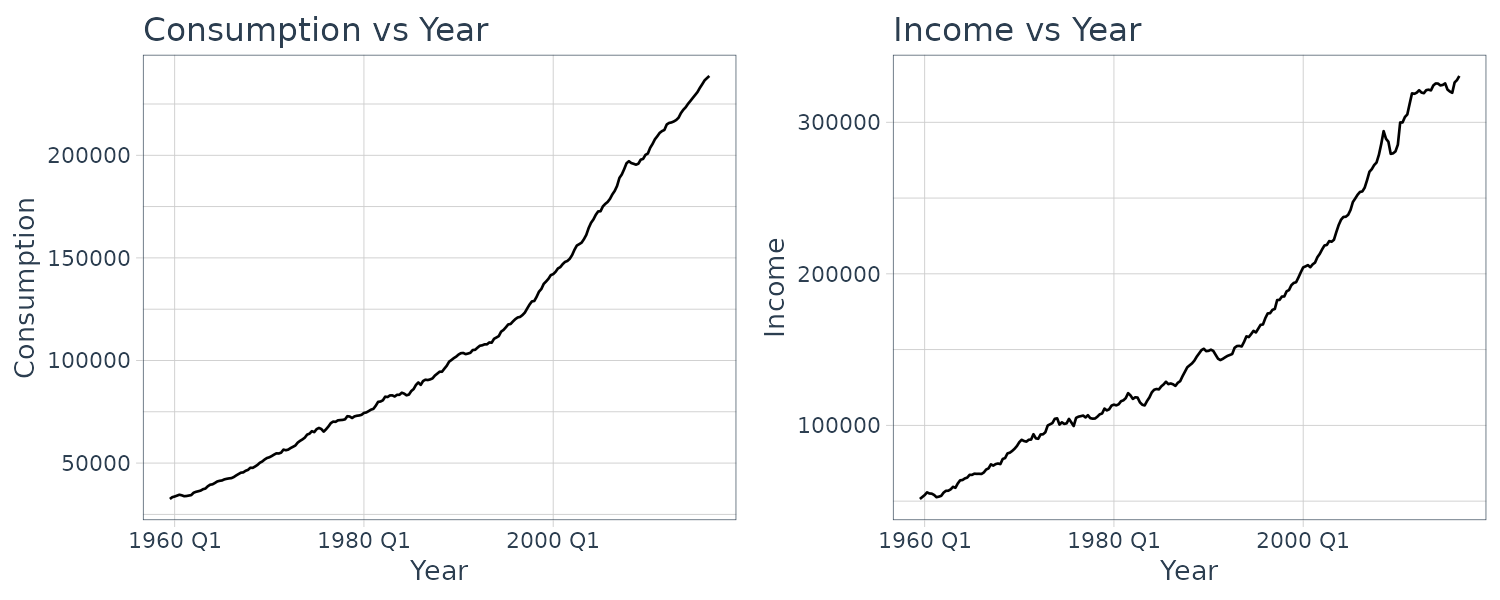
We can see that both variables are trending up. We first test if they are both trend stationary using the augmented Dickey-Fuller test to test for stationarity of the residuals:
fit <- lm(
  cons ~ t,
  data = cons_inc
)

> tseries::adf.test(fit$residuals)
	Augmented Dickey-Fuller Test

data:  fit$residuals
Dickey-Fuller = 0.16182, Lag order = 6, p-value = 0.99
alternative hypothesis: stationary

Warning message:
In adf.test(fit$residuals) : p-value greater than printed p-value

fit <- lm(
  y ~ t,
  data = cons_inc
)

> adf.test(fit$residuals)
	Augmented Dickey-Fuller Test

data:  fit$residuals
Dickey-Fuller = -0.73742, Lag order = 6, p-value = 0.966
alternative hypothesis: stationary
Both variables fails to reject the null hypothesis and are then shown to be not trend stationary. We next check if they are cointegrated:
fit <- lm(
  cons ~ t + y,
  data = cons_inc
)

> adf.test(fit$residuals)
	Augmented Dickey-Fuller Test

data:  fit$residuals
Dickey-Fuller = -0.73742, Lag order = 6, p-value = 0.966
alternative hypothesis: stationary

> fit <- lm(
+   cons ~ t + y,
+   data = cons_inc
+ )
+ adf.test(fit$residuals)
	Augmented Dickey-Fuller Test

data:  fit$residuals
Dickey-Fuller = -3.1158, Lag order = 6, p-value = 0.1072
alternative hypothesis: stationary
They are also not cointegrated. In this case, we take the first difference and fit the following ARDL model of \(C, Y\) in first differences:
fit <- lm(
  dc ~ dy + lag(dc),
  data = cons_inc
)

> summary(fit)
Call:
lm(formula = dc ~ dy + lag(dc), data = cons_inc)

Residuals:
     Min       1Q   Median       3Q      Max
-2415.77  -406.65   -70.98   452.18  2111.42

Coefficients:
             Estimate Std. Error t value Pr(>|t|)
(Intercept) 478.61146   74.19763   6.450 6.79e-10 ***
dy            0.09908    0.02154   4.599 7.09e-06 ***
lag(dc)       0.33690    0.05986   5.628 5.43e-08 ***
---
Signif. codes:  0 ‘***’ 0.001 ‘**’ 0.01 ‘*’ 0.05 ‘.’ 0.1 ‘ ’ 1

Residual standard error: 734.7 on 224 degrees of freedom
  (2 observations deleted due to missingness)
Multiple R-squared:  0.2214,	Adjusted R-squared:  0.2144
F-statistic: 31.85 on 2 and 224 DF,  p-value: 6.721e-13
Vector Autoregressive Models
Up till now, we have assumed that one of the variables \(y_{t}\) was the dependent variable and that the other \(x_{t}\) was the independent variable. However, apriori, unless we have good reasons not to, we could just as easily have assumed that \(y_{t}\) is the independent and \(x_{t}\) is the dependent variable:
\[\begin{aligned} y_{t} &= \beta_{10} + \beta_{11}y_{t-1} + \beta_{12}x_{t-1} + e_{yt}\\ x_{t} &= \beta_{20} + \beta_{21}y_{t-1} + \beta_{22}x_{t-1} + e_{xt}\\ \end{aligned}\] \[\begin{aligned} e_{yt} &\sim N(0, \sigma_{y}^{2})\\ e_{xt} &\sim N(0, \sigma_{x}^{2}) \end{aligned}\]In this bivariate (two series) system, there can be only one unique relationship between \(x_{t}\) and \(y_{t}\), and so it must be the case that:
\[\begin{aligned} \beta_{21} &= \frac{1}{\beta_{11}}\\ \beta_{20} &= -\frac{\beta_{10}}{\beta_{11}} \end{aligned}\]The above system can be estimated by least squares applied to each equation.
VEC and VAR Models
Let us start with only 2 variables \(x_{t}, y_{t}\). If \(y, x\) are stationary variables, we can use the following VAR(1) system of equations:
\[\begin{aligned} y_{t} &= \beta_{10} + \beta_{11}y_{t-1} + \beta_{12}x_{t-1} + v_{yt}\\ x_{t} &= \beta_{20} + \beta_{21}y_{t-1} + \beta_{22}x_{t-1} + v_{xt}\\ \end{aligned}\]If \(y, x\) are nonstationary I(1) and not cointegrated, then the VAR model is:
\[\begin{aligned} \Delta y_{t} &= \beta_{10} + \beta_{11}\Delta y_{t-1} + \beta_{12}\Delta x_{t-1} + v_{yt}\\ \Delta x_{t} &= \beta_{20} + \beta_{21}\Delta y_{t-1} + \beta_{22}\Delta x_{t-1} + v_{xt} \end{aligned}\]All variables are now I(0) and can be solved by least squares applied to each equation as before.
However, if \(y, x\) are conintegrated of order 1:
\[\begin{aligned} y_{t} &\sim I(1)\\ x_{t} &\sim I(1)\\ y_{t} &= \beta_{0} + \beta_{1}x_{t} + e_{t} \end{aligned}\]If y and x are I(1) and cointegrated, then we need to modify the system of equations to allow for the cointegrating relationship between the I(1) variables. Introducing the cointegrating relationship leads to a model known as the VEC model.
Consider two nonstationary variables \(y_{t}, x_{t}\) that are integrated of order 1 and are shown to be conintegrated:
\[\begin{aligned} y_{t} &= \beta_{0} + \beta_{1}x_{t} + e_{t} \end{aligned}\] \[\begin{aligned} y_{t} &\sim I(1)\\ x_{t} &\sim I(1)\\ \hat{e}_{t} &\sim I(0)\\ \end{aligned}\]The VEC model is:
\[\begin{aligned} \Delta y_{t} &= \alpha_{10} + \alpha_{11}(y_{t-1} - \beta_{0} - \beta_{1}x_{t-1}) + v_{yt}\\ \Delta x_{t} &= \alpha_{20} + \alpha_{21}(y_{t-1} - \beta_{0} - \beta_{1}x_{t-1}) + v_{xt} \end{aligned}\]Which can be expanded as:
\[\begin{aligned} y_{t} &= \alpha_{10} + (\alpha_{11} + 1)y_{t-1} - \alpha_{11}\beta_{0} - \alpha_{11}\beta_{1}x_{t-1} + v_{yt}\\ x_{t} &= \alpha_{20} + \alpha_{21}y_{t-1} - \alpha_{21}\beta_{0} - (\alpha_{21}\beta_{1} - 1)x_{t-1} + v_{xt} \end{aligned}\]Comparing the above with:
\[\begin{aligned} y_{t} &= \beta_{10} + \beta_{11}y_{t-1} + \beta_{12}x_{t-1} + v_{yt}\\ x_{t} &= \beta_{20} + \beta_{21}y_{t-1} + \beta_{22}x_{t-1} + v_{xt}\\ \end{aligned}\]Both equations depend on \(y_{t-1}, x_{t-1}\). The coefficients \(\alpha_{11}, \alpha_{22}\) are known as error correction coefficients.
The coefficients \(\alpha_{11}, \alpha_{21}\) are known as error correction coefficients, so named because they show how much \(\Delta y_{t}, \Delta x_{t}\) respond to the cointegrating error \(y_{t−1} – \beta_{0} – \beta_{1} x_{t-1} = e_{t-1}\). The idea that the error leads to (a correction comes about because) of the conditions put on \(\alpha_{11}, \alpha_{21}\) to ensure stability:
\[\begin{aligned} -1 < &\ \alpha_{11} \leq 0\\ 0 \leq &\ \alpha_{21} < 1 \end{aligned}\]To appreciate this idea, consider a positive error \(e_{t−1} > 0\) that occurred because \(y_{t−1} > \beta_{0} + \beta_{1} x_{t-1}\) . A negative error correction that \(\Delta y\) falls, while the positive error correction coefficient in the first equation \(\alpha_{11}\) ensures coefficient in the second equation \(\alpha_{21}\) ensures that \(\Delta x\) rises, thereby correcting the error. Having the error correction coefficients less than 1 in absolute value ensures that the system is not explosive. Note that the VEC is a generalization of the error-correction (single-equation) model discussed earlier.
The cointegration part measure how much y changes in response to x:
\[\begin{aligned} y_{t} &= \beta_{0} + \beta_{1}x_{t} + e_{t} \end{aligned}\]And the speed of the change (the error correction part):
\[\begin{aligned} \Delta y_{t} &= \alpha_{10} + \alpha_{11}(e_{t-1}) + v_{yt} \end{aligned}\]Note that the intercept terms (by grouping them):
\[\begin{aligned} y_{t} &= (\alpha_{10} - \alpha_{11}\beta_{0}) + (\alpha_{11} + 1)y_{t-1} - \alpha_{11}\beta_{1}x_{t-1} + v_{yt}\\ x_{t} &= (\alpha_{20} - \alpha_{21}\beta_{0}) + \alpha_{21}y_{t-1} - (\alpha_{21}\beta_{1} - 1)x_{t-1} + v_{xt} \end{aligned}\]If we estimate each equation by least squares, we obtain estimates of composite terms \((\alpha_{10} − \alpha_{11}\beta_{0}\) and \(\alpha_{20} - \alpha_{21}\beta_{0}\), and we are not able to disentangle the separate effects of \(\beta_{0}, \alpha_{10}, \alpha_{20}\). In the next section, we discuss a simple two-step least squares procedure that gets around this problem.
Estimating a Vector Error Correction Model
We could use a nonlinear least squares method, but a simpler way is to use a two-step least squares procedure. First, use OLS to estimate the cointegrating relationship:
\[\begin{aligned} \Delta y_{t} &= \beta_{0} + \beta_{1}x_{t} + e_{t}\\ \end{aligned}\]And generate the lagged residuals:
\[\begin{aligned} \hat{e}_{t-1} &= y_{t-1} - \hat{\beta}_{0} - \hat{\beta}_{1}x_{t-1} \end{aligned}\]Next use OLS to estimate:
\[\begin{aligned} \Delta y_{t} &= \alpha_{10} + \alpha_{11}\hat{e}_{t-1} + v_{yt}\\ \Delta x_{t} &= \alpha_{20} + \alpha_{21}\hat{e}_{t-1} + v_{xt} \end{aligned}\]Since all the variables are stationary, we can use the standard regression analysis to test the significance of the parameters.
Example: VEC Model for GDP
Below shows the plot of Australia and US real GDP:
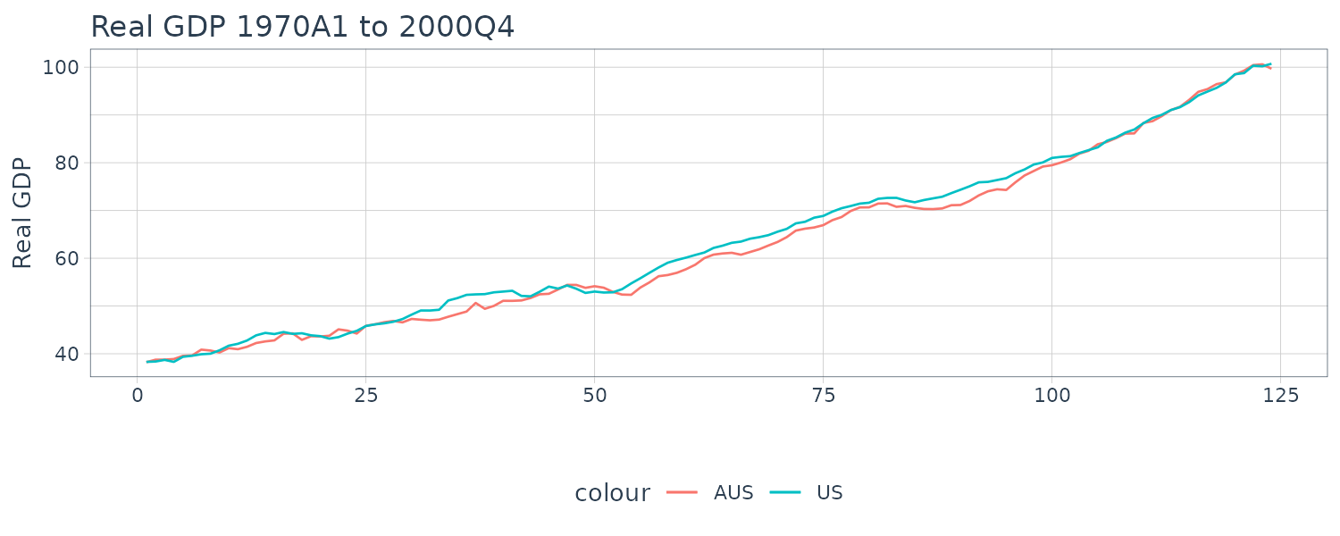
It appears that both series are nonstationary and possibly cointegrated.
Checking if the residuals are stationary:
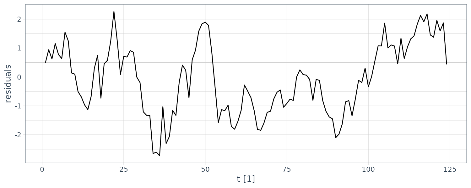
> gdp |>
  features(
    residuals,
    unitroot_pp
  )
# A tibble: 1 × 2
  pp_stat pp_pvalue
    <dbl>     <dbl>
1   -2.96    0.0453
As the p-value is significant, we can conclude the residuals are stationary. Next, we do a cointegration fit with no intercept:
fit <- lm(
  aus ~ 0 + usa,
  data = gdp
)

> summary(fit)
Call:
lm(formula = aus ~ 0 + usa, data = gdp)

Residuals:
     Min       1Q   Median       3Q      Max
-2.72821 -1.06932 -0.08543  0.91592  2.26603

Coefficients:
    Estimate Std. Error t value            Pr(>|t|)
usa 0.985350   0.001657   594.8 <0.0000000000000002 ***
---
Signif. codes:  0 ‘***’ 0.001 ‘**’ 0.01 ‘*’ 0.05 ‘.’ 0.1 ‘ ’ 1

Residual standard error: 1.219 on 123 degrees of freedom
Multiple R-squared:  0.9997,	Adjusted R-squared:  0.9996
F-statistic: 3.538e+05 on 1 and 123 DF, p-value: < 0.00000000000000022 If \(U_{t}\) were to increase by one unit, \(A_{t}\) would increase by 0.985. But the Australian economy may not respond fully by this amount within the quarter. To ascertain how much it will respond within a quarter, we estimate the error correction by least squares.
The estimated VEC model for \(A_{t}, U_{t}\) is:
gdp$diff_aus <- c(NA, diff(gdp$aus))
gdp$diff_usa <- c(NA, diff(gdp$usa))

fit1 <- lm(
  diff_aus ~ lag(residuals),
  data = gdp
)

> summary(fit1)
Call:
lm(formula = diff_aus ~ lag(residuals), data = gdp)

Residuals:
     Min       1Q   Median       3Q      Max
-1.82072 -0.41633  0.01881  0.41823  1.73368

Coefficients:
               Estimate Std. Error t value           Pr(>|t|)
(Intercept)     0.49171    0.05791   8.491 0.0000000000000612 ***
lag(residuals) -0.09870    0.04752  -2.077             0.0399 *
---
Signif. codes:  0 ‘***’ 0.001 ‘**’ 0.01 ‘*’ 0.05 ‘.’ 0.1 ‘ ’ 1

Residual standard error: 0.6409 on 121 degrees of freedom
  (1 observation deleted due to missingness)
Multiple R-squared:  0.03443,	Adjusted R-squared:  0.02645
F-statistic: 4.315 on 1 and 121 DF,  p-value: 0.03989

fit2 <- lm(
  diff_usa ~ lag(residuals),
  data = gdp
)

> summary(fit2)
Call:
lm(formula = diff_usa ~ lag(residuals), data = gdp)

Residuals:
     Min       1Q   Median       3Q      Max
-1.54329 -0.30388  0.03483  0.36117  1.47005

Coefficients:
               Estimate Std. Error t value            Pr(>|t|)
(Intercept)     0.50988    0.04668   10.92 <0.0000000000000002 ***
lag(residuals)  0.03025    0.03830    0.79               0.431
---
Signif. codes:  0 ‘***’ 0.001 ‘**’ 0.01 ‘*’ 0.05 ‘.’ 0.1 ‘ ’ 1

Residual standard error: 0.5166 on 121 degrees of freedom
  (1 observation deleted due to missingness)
Multiple R-squared:  0.005129,	Adjusted R-squared:  -0.003093
F-statistic: 0.6238 on 1 and 121 DF, p-value: 0.4312The results show that both error correction coefficients are of the appropriate sign. The negative error correction coefficient in the first equation (−0.099) indicates that \(\Delta A\) falls, while the positive error correction coefficient in the second equation (0.030) indicates that \(\Delta U\) rises, when there is a positive cointegrating error (\(\hat{e}_{t−1} > 0\) or \(A_{t-1} > 0.985 U_{t-1}\)). This behavior (negative change in A and positive change in U) “corrects” the cointegrating error.
The error correction coefficient (−0.099) is significant at the 5% level; it indicates that the quarterly adjustment of \(A_{t}\) will be about 10% of the deviation of \(A_{t−1}\) from its cointegrating value \(0.985U_{t−1}\). This is a slow rate of adjustment.
However, the error correction coefficient in the second equation (0.030) is insignificant; it suggests that \(\Delta U\) does not react to the cointegrating error. This outcome is consistent with the view that the small economy is likely to react to economic conditions in the large economy, but not vice versa.
Estimating a VAR Model
What if \(y, x\) are not cointegrated? In this case, we estimate VAR model.
Example: VAR Model for Consumption and Income
Using the dataset fred5:
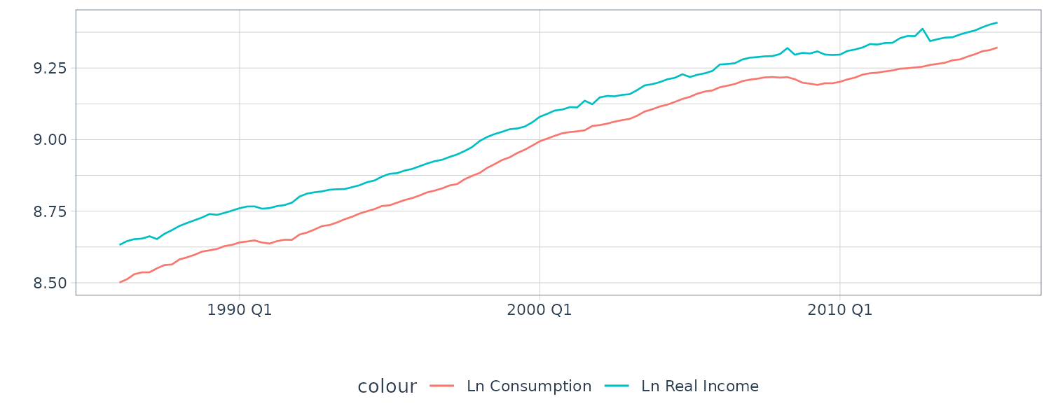
The plot shows the log of real personal disposable income (RPDI) (denoted as Y) and the log of real personal consumption expenditure (RPCE) (denoted as C) for the U.S. economy over the period 1986Q1 to 2015Q2. Both series appear to be nonstationary, but are they cointegrated?
Testing for unitroot, it shows the residuals are stationary. But not the augmented Dickey Fuller test:
> fred5 |>
  features(
    residuals,
    unitroot_pp
  )
# A tibble: 1 × 2
  pp_stat pp_pvalue
    <dbl>     <dbl>
1   -4.29      0.01

> tseries::adf.test(fit$residuals)
	Augmented Dickey-Fuller Test

data:  fit$residuals
Dickey-Fuller = -2.8349, Lag order = 4, p-value = 0.2299
alternative hypothesis: stationary
Assuming the residuals are not stationary, we conclude there is no cointegration. Thus, we would not apply a VEC model to examine the dynamic relationship between aggregate consumption C and income Y. Instead, we would estimate a VAR model for the set of I(0) variables:
fred5$diff_consn <- c(NA, diff(fred5$consn))
fred5$diff_y <- c(NA, diff(fred5$y))

fit1 <- lm(
  diff_consn ~ lag(diff_consn) + lag(diff_y),
  data = fred5
)

> summary(fit1)
Call:
lm(formula = diff_consn ~ lag(diff_consn) +
  lag(diff_y), data = fred5)

Residuals:
       Min         1Q     Median         3Q        Max
-0.0142469 -0.0033214  0.0000404  0.0032337  0.0139020

Coefficients:
                 Estimate Std. Error t value   Pr(>|t|)
(Intercept)     0.0036707  0.0007532   4.873 0.00000361 ***
lag(diff_consn) 0.3481916  0.0865886   4.021   0.000105 ***
lag(diff_y)     0.1313454  0.0520669   2.523   0.013040 *
---
Signif. codes:  0 ‘***’ 0.001 ‘**’ 0.01 ‘*’ 0.05 ‘.’ 0.1 ‘ ’ 1

Residual standard error: 0.004736 on 113 degrees of freedom
  (2 observations deleted due to missingness)
Multiple R-squared:  0.2108,	Adjusted R-squared:  0.1969
F-statistic: 15.09 on 2 and 113 DF,  p-value: 0.00000155

fit2 <- lm(
  diff_y ~ lag(diff_consn) + lag(diff_y),
  data = fred5
)

> summary(fit2)
Call:
lm(formula = diff_y ~ lag(diff_consn) +
  lag(diff_y), data = fred5)

Residuals:
      Min        1Q    Median        3Q       Max
-0.041706 -0.003686 -0.000100  0.003810  0.019817

Coefficients:
                 Estimate Std. Error t value Pr(>|t|)
(Intercept)      0.004384   0.001295   3.384 0.000982 ***
lag(diff_consn)  0.589538   0.148918   3.959 0.000132 ***
lag(diff_y)     -0.290937   0.089546  -3.249 0.001526 **
---
Signif. codes:  0 ‘***’ 0.001 ‘**’ 0.01 ‘*’ 0.05 ‘.’ 0.1 ‘ ’ 1

Residual standard error: 0.008145 on 113 degrees of freedom
  (2 observations deleted due to missingness)
Multiple R-squared:  0.1555,	Adjusted R-squared:  0.1406
F-statistic: 10.4 on 2 and 113 DF, p-value: 0.00007118The first equation shows that the quarterly growth in consumption \(\Delta C_{t}\) is significantly related to its own past value \(\Delta C_{t−1}\) and also significantly related to the quarterly growth in last period’s income \(\Delta Y_{t-1}\).
The second equation shows that \(\Delta Y_{t}\) is significantly negatively related to its own past value but significantly positively related to last period’s change in consumption. The constant terms capture the fixed component in the change in log consumption and the change in log income.
The constant terms capture the fixed component in the change in log consumption and the change in log income.
Impulse Response Functions
Impulse response functions show the effects of shocks on the adjustment path of the variables.
Let us consider the impulse response function analysis with two time series on a bivariate VAR system of stationary variables:
\[\begin{aligned} y_{t} &= \delta_{10} + \delta_{11}y_{t-1} + \delta_{12}x_{t-1} + v_{yt}\\ x_{t} &= \delta_{20} + \delta_{21}y_{t-1} + \delta_{22}x_{t-1} + v_{xt} \end{aligned}\]There are 2 possible shocks to the system. One on y and another one on x. There are 4 impulse response functions, the effect on time-paths of x and y due to shock on y and the effect on time-paths of x and y due to shock on x.
We are assuming there is no contemporaneous relationship and hence no identification problem. This special case occurs when the system that is described above is a true representation of the dynamic system—namely, y is related only to lags of y and x, and x is related only to lags of y and x. In other words, y and x are related dynamically, but not contemporaneously. The current value xt does not appear in the equation for \(y_{t}\) and the current value \(y_{t}\) does not appear in the equation for \(x_{t}\). Also, we need to assume that the errors \(v_{tx}\) and \(v_{ty}\) are contemporaneously uncorrelated.
Consider the case when there is a one standard deviation shock (innovation) to y so that at time \(t = 1\), \(v_{1y} = \sigma_{y}\) , and \(v_{t}\) is zero thereafter. Assume \(v_{tx} = 0\) for all t. Assume \(y_{0} = x_{0} = 0\). Also, since we are focusing on how a shock changes the paths of y and x, we can ignore the intercepts.
Consider at \(t=1\), there is a \(\sigma_{y}\) shock on \(y\):
\[\begin{aligned} y_{0} &= 0\\ x_{0} &= 0\\ y_{1} &= v_{1y}\\ &= \sigma_{y}\\ x_{1} &= 0 \end{aligned}\] \[\begin{aligned} y_{2} &= \delta_{11}y_{1} + \delta_{12}x_{1}\\ &= \delta_{11}\sigma_{y} + \delta_{12}0\\ &= \delta_{11}\sigma_{y}\\ x_{2} &= \delta_{21}y_{1} + \delta_{22}x_{1}\\ &= \delta_{21}\sigma_{y} + \delta_{22}0\\ &= \delta_{21}\sigma_{y}\\ y_{3} &= \delta_{11}\delta_{11}\sigma_{y} + \delta_{12}\delta_{21}\sigma_{y}\\ x_{3} &= \delta_{21}\delta_{11}\sigma_{y} + \delta_{22}\delta_{21}\sigma_{y}\\ &\ \ \vdots \end{aligned}\]The impulse response of the shock (or innovation) to y on y is:
\[\begin{aligned} \sigma_{y}[1, \delta_{11}, \delta_{11}\delta_{11} + \delta_{12}\delta_{21}, \cdots] \end{aligned}\]The impulse response to y on x is:
\[\begin{aligned} \sigma_{y}[0, \delta_{21}, \delta_{21}\delta_{11} + \delta_{22}\delta_{21}, \cdots] \end{aligned}\]Now consider a shock of \(\sigma_{x}\) on \(x\):
\[\begin{aligned} y_{0} &= 0\\ x_{0} &= 0\\ x_{1} &= v_{1x}\\ &= \sigma_{x}\\ y_{1} &= 0 \end{aligned}\] \[\begin{aligned} y_{2} &= \delta_{11}y_{1} + \delta_{12}x_{1}\\ &= \delta_{11}0 + \delta_{12}\sigma_{x}\\ &= \delta_{12}\sigma_{x}\\ x_{2} &= \delta_{21}y_{1} + \delta_{22}x_{1}\\ &= \delta_{21}0 + \delta_{22}\sigma_{x}\\ &= \delta_{22}\sigma_{x}\\ &\ \ \vdots \end{aligned}\]The impulse response to x on y is:
\[\begin{aligned} \sigma_{x}[0, \delta_{12}, \delta_{11}\delta_{12} + \delta_{12}\delta_{22}, \cdots] \end{aligned}\]The impulse response to x on x is:
\[\begin{aligned} \sigma_{x}[1, \delta_{22}, \delta_{21}\delta_{12} + \delta_{22}\delta_{22}, \cdots] \end{aligned}\]The advantage of examining impulse response functions on top of VAR coefficients is that they show the size of the impact of the shock plus the rate at which the shock dissipates.
Forecast Error Variance Decompositions
The one-step ahead forecasts are:
\[\begin{aligned} y_{t+1}^{F} &= E_{t}[\delta_{11}y_{t} + \delta_{12}x_{t} + \nu_{t+1}^{y}]\\ &= \delta_{11}y_{t} + \delta_{12}x_{t}\\[5pt] x_{t+1}^{F} &= E_{t}[\delta_{21}y_{t} + \delta_{22}x_{t} + \nu_{t+1}^{x}]\\ &= \delta_{12}y_{t} + \delta_{22}x_{t}\\[5pt] \end{aligned}\]The forecast errors:
\[\begin{aligned} \text{FE}_{1}^{y} &= y_{t+1} - E_{t}[y_{t+1}]\\ &= \nu_{t+1}^{y}\\ \text{FE}_{1}^{x} &= x_{t+1} - E_{t}[x_{t+1}]\\ &= \nu_{t+1}^{x} \end{aligned}\]And the variances:
\[\begin{aligned} \text{var}(\text{FE}_{1}^{y}) &= \sigma_{y}^{2}\\ \text{var}(\text{FE}_{1}^{x}) &= \sigma_{x}^{2}\\ \end{aligned}\]All variation in the forecast for \(y\) is due to its own shock and the same for the forecast for \(x\) is due to its own shock.
For the two-step forecast:
\[\begin{aligned} y_{t+2}^{F} &= E_{t}[\delta_{11}y_{t+1} + \delta_{12}x_{t+1} + \nu_{t+2}^{y}]\\ &= E_{t}[\delta_{11}(\delta_{11}y_{t} + \delta_{12}x_{t} + \nu_{t+1}^{y}) + \delta_{12}(\delta_{21}y_{t} + \delta_{22}x_{t} + \nu_{t+1}^{x}) + \nu_{t+2}^{y}]\\ &= \delta_{11}(\delta_{11}y_{t} + \delta_{12}x_{t}) + \delta_{12}(\delta_{21}y_{t} + \delta_{22}x_{t}) \end{aligned}\] \[\begin{aligned} x_{t+2}^{F} &= E_{t}[\delta_{21}y_{t+1} + \delta_{22}x_{t+1} + \nu_{t+2}^{x}]\\ &= E_{t}[\delta_{21}(\delta_{11}y_{t} + \delta_{12}x_{t} + \nu_{t+1}^{y}) + \delta_{22}(\delta_{21}y_{t} + \delta_{22}x_{t} + \nu_{t+1}^{x}) + \nu_{t+2}^{y}]\\ &= \delta_{21}(\delta_{11}y_{t} + \delta_{12}x_{t}) + \delta_{22}(\delta_{21}y_{t} + \delta_{22}x_{t}) \end{aligned}\]The two-step forecast errors:
\[\begin{aligned} \text{FE}_{2}^{y} &= y_{t+2} - E_{t}[y_{t+2}]\\ &= \delta_{11}(\delta_{11}y_{t} + \delta_{12}x_{t} + \nu_{t+1}^{y}) + \delta_{12}(\delta_{21}y_{t} + \delta_{22}x_{t} + \nu_{t+1}^{x}) + \nu_{t+2}^{y} - y_{t+2}^{F}\\ &= \delta_{11}\nu_{t+1}^{y} + \delta_{12}\nu_{t+1}^{x} + \nu_{t+2}^{y}\\[5pt] \text{FE}_{2}^{x} &= x_{t+2} - E_{t}[x_{t+2}]\\ &= \delta_{21}(\delta_{11}y_{t} + \delta_{22}x_{t} + \nu_{t+1}^{y}) + \delta_{22}(\delta_{21}y_{t} + \delta_{22}x_{t} + \nu_{t+1}^{x}) + \nu_{t+2}^{x} - x_{t+2}^{F}\\ &= \delta_{21}\nu_{t+1}^{y} + \delta_{22}\nu_{t+1}^{x} + \nu_{t+2}^{x} \end{aligned}\]And the forecast variances:
\[\begin{aligned} \text{var}(\text{FE}_{2}^{y}) &= \delta_{11}^{2}\sigma_{y}^{2} + \delta_{12}\sigma_{x}^{2} + \sigma_{y}^{2}\\ \text{var}(\text{FE}_{2}^{x}) &= \delta_{21}^{2}\sigma_{y}^{2} + \delta_{22}\sigma_{x}^{2} + \sigma_{x}^{2} \end{aligned}\]We can decompose the total variance of the forecast error for \(y\) due to shocks to \(y\):
\[\begin{aligned} \delta_{11}^{2}\sigma_{y}^{2} + \delta_{12}\sigma_{x}^{2} + \sigma_{y}^{2} \end{aligned}\]And shocks to \(x\):
\[\begin{aligned} \delta_{12}\sigma_{x}^{2} \end{aligned}\]To see the proportion of shocks:
Proportion of error variance of \(y\) explained by its own shock is:
\[\begin{aligned} \frac{\delta_{11}^{2}\sigma_{y}^{2} + \sigma_{y}^{2}}{\delta_{11}^{2}\sigma_{y}^{2} + \sigma_{12}^{2}\sigma_{x}^{2} + \sigma_{y}^{2}} \end{aligned}\]Proportion error variance of \(y\) explained by its other shock is:
\[\begin{aligned} \frac{\delta_{12}^{2}\sigma_{x}^{2}}{\delta_{11}^{2}\sigma_{y}^{2} + \sigma_{12}^{2}\sigma_{x}^{2} + \sigma_{y}^{2}} \end{aligned}\]Proportion of error variance of \(x\) explained by its own shock is:
\[\begin{aligned} \frac{\delta_{22}^{2}\sigma_{x}^{2} + \sigma_{x}^{2}}{\delta_{21}^{2}\sigma_{y}^{2} + \sigma_{22}^{2}\sigma_{x}^{2} + \sigma_{x}^{2}} \end{aligned}\]Proportion error variance of $x$$ explained by its other shock is:
\[\begin{aligned} \frac{\delta_{21}^{2}\sigma_{y}^{2}}{\delta_{21}^{2}\sigma_{y}^{2} + \sigma_{22}^{2}\sigma_{x}^{2} + \sigma_{x}^{2}} \end{aligned}\]In summary, a VAR model model will tell you whether the variables are significantly related to each other. An impulse response analysis will show how the variables react dynamically to shocks. Finally, a variance decomposition analysis will show the sources of volatility.
ARCH Models
We were concerned with stationary and nonstationary variables, and, in particular, macroeconomic variables like gross domestic product (GDP), inflation, and interest rates. The nonstationary nature of the variables implied that they had means that change over time. In this chapter, we are concerned with stationary series, but with conditional variances that change over time. The model we focus on is called the autoregressive conditional heteroskedastic (ARCH) model.
ARCH stands for autoregressive conditional heteroskedasticity. We have covered the concepts of autoregressive and heteroskedastic errors.
Consider a model with an AR(1) error term:
\[\begin{aligned} y_{t} &= \phi + e_{t}\\ e_{t} &= \rho e_{t-1} + v_{t} \end{aligned}\] \[\begin{aligned} |\rho| &< 1\\ v_{t} &\sim N(0, \sigma_{v}^{2}) \end{aligned}\]For convenience of exposition, first perform some successive substitution to obtain \(e_{t}\) as the sum of an infinite series of the error term \(v_{t}\):
\[\begin{aligned} e_{t} &= \rho e_{t-1} + v_{t}\\ e_{t} &= \rho (\rho e_{t-2} + v_{t-1}) + v_{t}\\ &\ \ \vdots\\ e_{t} &= v_{t} + \rho^{2}v_{t-2} + \cdots + \rho^{t}e_{0} \end{aligned}\]The unconditional mean for the error (having no info):
\[\begin{aligned} E[e_{t}] &= E[v_{t} + \rho^{2}v_{t-2} + \cdots + \rho^{t}e_{0}]\\ &= 0 \end{aligned}\]While the conditional mean for the error, conditional on information prior to time \(t\):
\[\begin{aligned} E[e_{t}|I_{t-1}] &= E[\rho e_{t-1} + v_{t} | I_{t-1}]\\ &= E[\rho e_{t-1}|I_{t-1}] + E[v_{t}]\\ &= E[\rho e_{t-1}|I_{t-1}] + 0\\ &= \rho e_{t-1} \end{aligned}\]The information set at time \(t − 1\), \(I_{t−1}\), includes knowing \(\rho e_{t−1}\). Put simply, “unconditional” describes the situation when you have no information, whereas conditional describes the situation when you have information, up to a certain point in time.
The unconditional variance of the error:
\[\begin{aligned} E\Big[e_{t} - E[e_{t}]\Big]^{2} &= E[e_{t} - 0]^{2}\\ &= E[v_{t} + \rho v_{t-1} + \rho^{2}v_{t-2} + \cdots]^{2}\\ &= E[v_{t}^{2} + \rho^{2}v_{t-1}^{2} + \rho^{4}v_{t-2}^{2} + \cdots]\\ &= \sigma_{v}^{2}(1 + \rho^{2} + \rho^{4} + \cdots)\\ &= \frac{\sigma_{v}^{2}}{1 - \rho^{2}} \end{aligned}\] \[\begin{aligned} E[v_{t-j}v_{t-i}] &= 0\\ i &\neq j \end{aligned}\]The conditional variance is:
\[\begin{aligned} E\Big[(e_{t} - E[e_{t}|I_{t-1}])^{2}|I_{t-1}\Big] &= E[(e_{t} - \rho e_{t-1})^{2}|I_{t-1}]\\ &= E[v_{t}|I_{t-1}]\\ &= \sigma_{v}^{2} \end{aligned}\]Now notice, for this model, that the conditional mean of the error varies over time, while the conditional variance does not. Suppose that instead of a conditional mean that changes over time, we have a conditional variance that changes over time. To introduce this modification, consider a variant of the above model:
\[\begin{aligned} y_{t} &= \beta_{0} + e_{t}\\ e_{t}|I_{t-1} &\sim N(0, h_{t})\\ h_{t} &= \alpha_{0} + \alpha_{1}e_{t-1}^{2} \end{aligned}\] \[\begin{aligned} \alpha_{0} &> 0 \end{aligned}\] \[\begin{aligned} 0 \leq \alpha_{1} < 1 \end{aligned}\]The name ARCH conveys the fact that we are working with time-varying variances (heteroskedasticity) that depend on (are conditional on) lagged effects (autocorrelation). This particular example is an ARCH(1) model since the time-varying variance \(h_{t}\) is a function of a constant term \(\alpha_{0}\) plus a term lagged once, the square of the error in the previous period \(\alpha_{1}e_{t−1}^{2}\). The coefficients, \(\alpha_{0}, \alpha_{1}\), have to be positive to ensure a positive variance.
The coefficient \(\alpha_{1}\) must be less than 1, or \(h_{t}\) will continue to increase over time, eventually exploding. Conditional normality means that the normal distribution is a function of known information at time \(t − 1\); i.e., when \(t = 2\), \(e2 \mid I1 \sim N(0, \alpha_{0} + \alpha_{1} e_{1}^{2})\) and so on. In this particular case, conditioning on \(I_{t−1}\) is equivalent to conditioning on the square of the error in the previous period \(e_{t−1}^{2}\).
Note that while the conditional distribution of the error \(e_{t}\) is assumed to be normal, the unconditional distribution of the error \(e_{t}\) will not be normal. This is not an inconsequential consideration given that a lot of real-world data appear to be drawn from non-normal distributions.
We can standardized the errors to be standard normal:
\[\begin{aligned} z_{t} &= \frac{e_{t}}{\sqrt{h_{t}}}\Big| I_{t-1}\\[5pt] &\sim N(0, 1) \end{aligned}\]Note that \(z_{t}\) and \(e_{t-1}^{2}\) are independent. Thus:
\[\begin{aligned} E[e_{t}] &= E\Big[\frac{e_{t}}{\sqrt{h_{t}}} \times \sqrt{h_{t}}\Big]\\ &= E\Big[\frac{e_{t}}{\sqrt{h_{t}}}\Big] \times E[\sqrt{h_{t}}]\\ &= E[z_{t}]E[\sqrt{\alpha_{0} + \alpha_{1}e_{t-1}^{2}}]\\ &= 0 \times E[\sqrt{\alpha_{0} + \alpha_{1}e_{t-1}^{2}}]\\ &= 0\\ E[e_{t}^{2}] &= E[z_{t}^{2}]E[\alpha_{0} + \alpha_{1}e_{t-1}^{2}]\\ &= \alpha_{0} + \alpha_{1}E[e_{t-1}^{2}]\\ &= \alpha_{0} + \alpha_{1}E[e_{t}^{2}] \end{aligned}\] \[\begin{aligned} E[e_{t}^{2}] - \alpha_{1}E[e_{t}^{2}] &= \alpha_{0}\\ E[e_{t}^{2}](1 - \alpha_{1}) &= \alpha_{0} \end{aligned}\] \[\begin{aligned} E[e_{t}^{2}] &= \frac{\alpha_{0}}{1 - \alpha_{1}} \end{aligned}\]The ARCH model has become a very important econometric model because it is able to capture stylized features of real-world volatility. Furthermore, in the context of the ARCH(1) model, knowing the squared error in the previous period \(e_{t−1}^{2}\) improves our knowledge about the likely magnitude of the variance in period t. This is useful for situations when it is important to understand risk, as measured by the volatility of the variable.
The ARCH model has become a popular one because its variance specification can capture commonly observed features of the time series of financial variables; in particular, it is useful for modeling volatility and especially changes in volatility over time. To appreciate what we mean by volatility and time-varying volatility, and how it relates to the ARCH model, let us look at some stylized facts about the behavior of financial variables—for example, the returns to stock price indices (also known as share price indices).
Example: Characteristics of Financial Variables
The plots shows the time series of the monthly returns to a number of stock prices; namely, the U.S. Nasdaq, the Australian All Ordinaries, the Japanese Nikkei, and the UK FTSE over the period 1988M1 to 2015M12 (data file returns5).
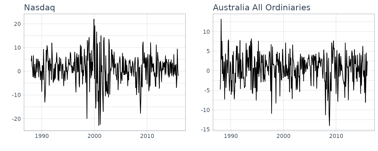
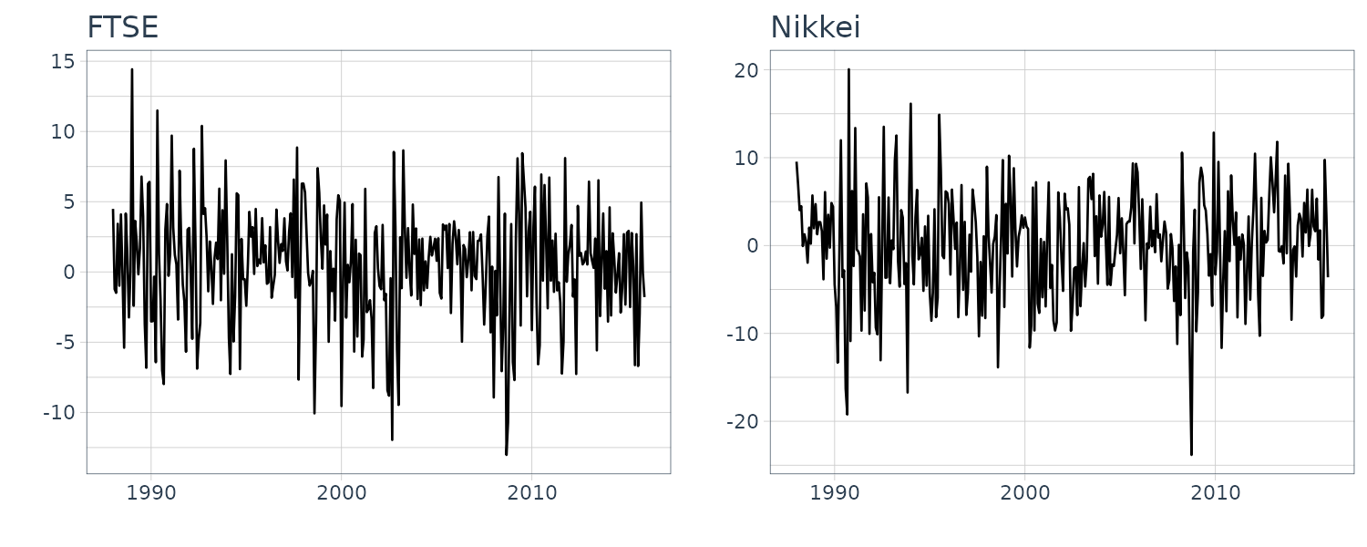
The values of these series change rapidly from period to period in an apparently unpredictable manner; we say the series are volatile. Furthermore, there are periods when large changes are followed by further large changes and periods when small changes are followed by further small changes. In this case the series are said to display time-varying volatility as well as “clustering” of changes.
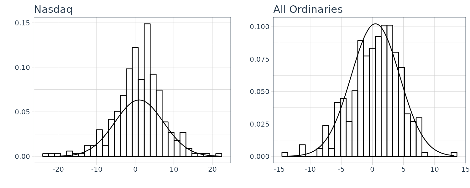
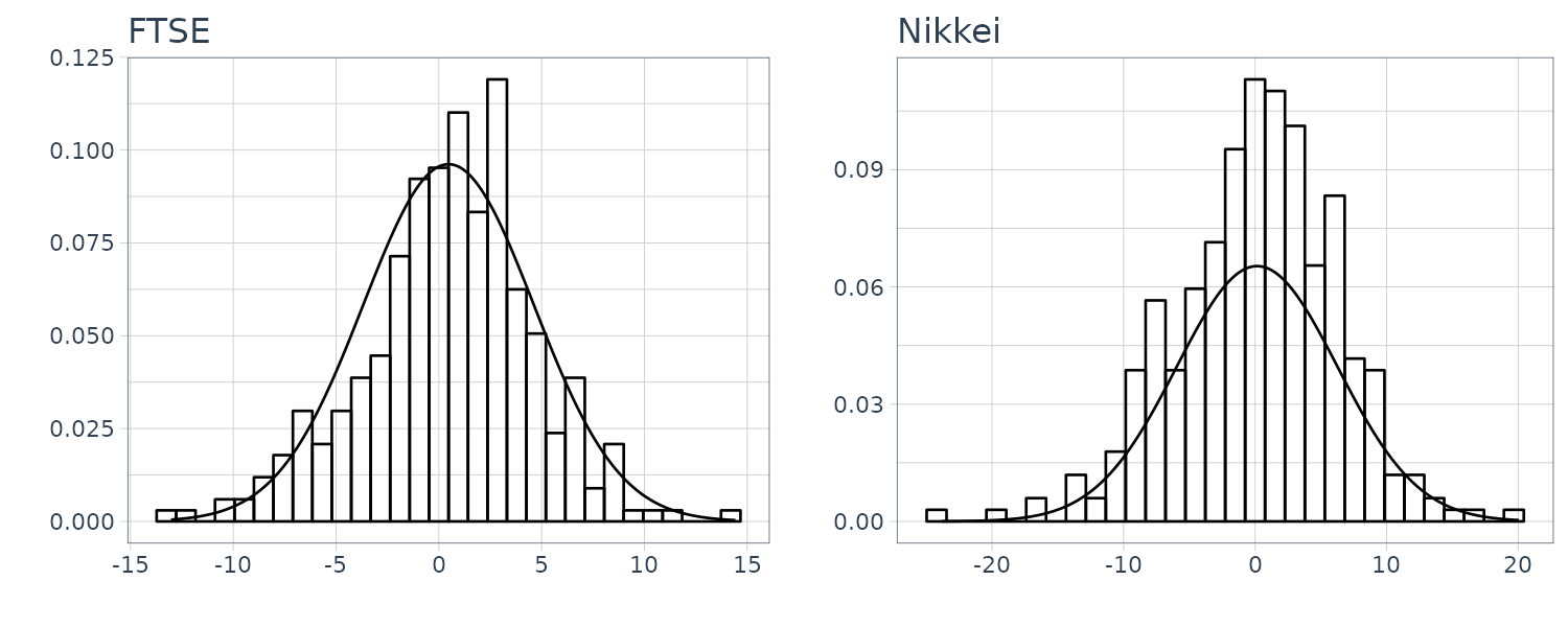
The above shows the histograms of the returns. All returns display non-normal properties. We can see this more clearly if we draw normal distributions on top of these histograms. Note that there are more observations around the mean and in the tails. Distributions with these properties more peaked around the mean and relatively fat tails are said to be leptokurtic.
Note the assumption that the conditional distribution for \(y_{t} \mid I_{t−1}\) is normal, an assumption that we made in, does not necessarily imply that the unconditional distribution for \(y_{t}\) is normal. What we have observed is that the unconditional distribution for \(y_{t}\) is leptokurtic.
Simulating Time-Varying Volatility
To illustrate how the ARCH model can be used to capture changing volatility and the leptokurtic nature of the distribution for \(y_{t}\), we generate some simulated data for two models.
In the first model, we set:
\[\begin{aligned} \beta_{0} &= 0\\ \alpha_{0} &= 1\\ \alpha_{1} &= 0 \end{aligned}\]This implies that:
\[\begin{aligned} y_{t} &= \beta_{0} + e_{t}\\ &= e_{t}\\ \textrm{var}(y_{t}|I_{t-1}) &= h_{t}\\ &= 1 + 0\times e_{t-1}^{2}\\ &= 1 \end{aligned}\]The variance is constant.
The next model, we set:
\[\begin{aligned} \beta_{0} &= 0\\ \alpha_{0} &= 1\\ \alpha_{1} &= 0.8 \end{aligned}\]This implies that:
\[\begin{aligned} y_{t} &= \beta_{0} + e_{t}\\ &= e_{t}\\ \textrm{var}(y_{t}|I_{t-1}) &= h_{t}\\ &= 1 + 0.8 e_{t-1}^{2} \end{aligned}\]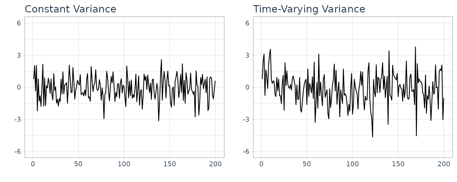
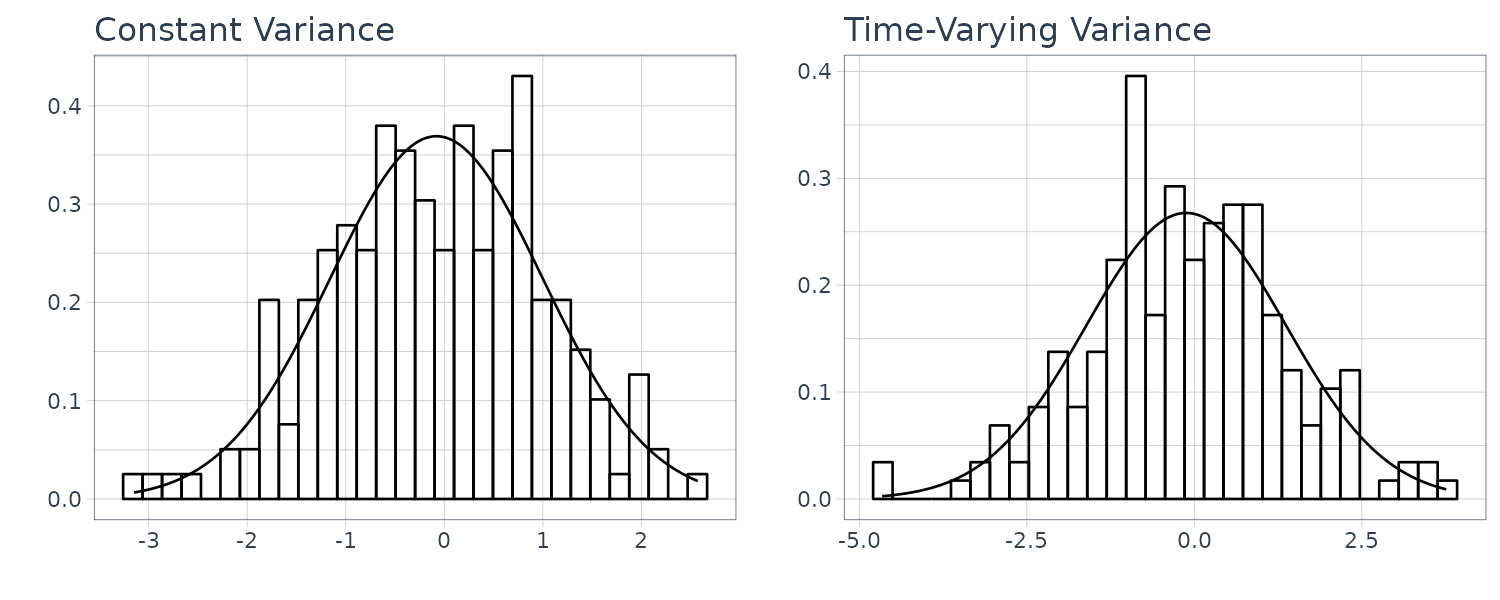
Thus, the ARCH model is intuitively appealing because it seems sensible to explain volatility as a function of the errors \(e_{t}\). These errors are often called “shocks” or “news” by financial analysts. They represent the unexpected! According to the ARCH model, the larger the shock, the greater the volatility in the series. In addition, this model captures volatility clustering, as big changes in \(e_{t}\) are fed into further big changes in ht via the lagged effect \(e_{t−1}\).
A Lagrange multiplier (LM) test is often used to test for the presence of ARCH effects. To perform this test, first estimate the mean equation, which can be a regression of the variable on a constant or may include other variables. To test for first-order ARCH:
\[\begin{aligned} \hat{e}_{t}^{2} &= \gamma_{0} + \gamma_{1}\hat{e}_{t-1}^{2} + v_{t} \end{aligned}\]The hypotheses are:
\[\begin{aligned} H_{0}:&\ \gamma_{1} = 0 H_{1}:&\ \gamma_{1} \neq 0 \end{aligned}\]If there are no ARCH effects, then \(\gamma_{1} = 0\). The LM test statistic is:
\[\begin{aligned} (T - q)R^{2} \end{aligned}\]If the null hypothesis is true, then the test statistic is distributed (in large samples) as \(\chi^{2}(q)\), where \(q\) is the order of lag, and \((T − q)\) is the number of complete observations. If \((T − q)R^{2} \geq \chi^{2}_{(1 - \alpha, q)}\), then we reject the null hypothesis that \(\gamma_{1} = 0\) and conclude that ARCH effects are present.
Example: Testing for ARCH in BrightenYourDay (BYD) Lighting
To illustrate the test, consider the returns from buying shares in the hypothetical company BYD Lighting.
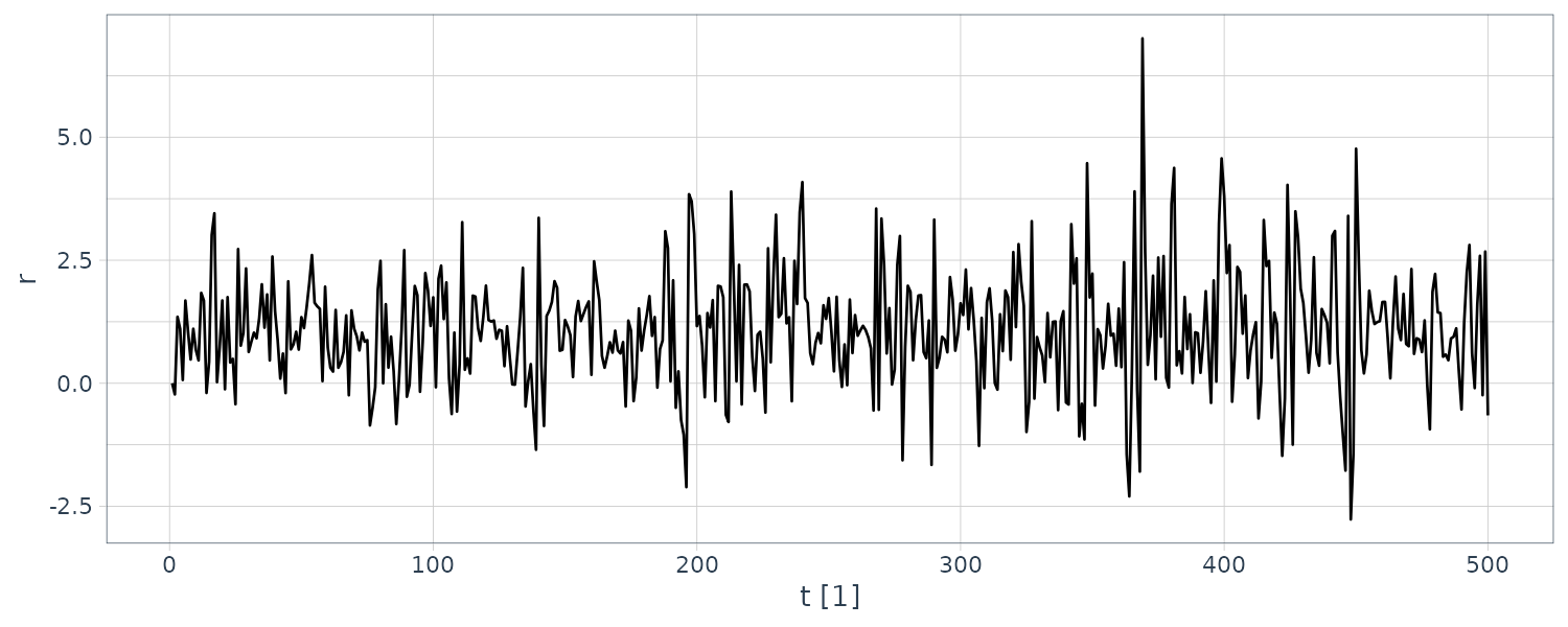
The time series shows evidence of time-varying volatility and clustering, and the unconditional distribution is non-normal.
To perform the test for ARCH effects:
\[\begin{aligned} \hat{e}_{t} &= 0.908 + 0.353\hat{e}_{t-1}^{2}\\ R^{2} &= 0.124 \end{aligned}\]The t-statistic suggests a significant first-order coefficient. The sample size is 500, giving an LM test value of:
\[\begin{aligned} (T − q)R^{2} &= (500 - 1)\times 0.124\\ &= 61.876 \end{aligned}\]Given \(\chi^{2}_{(0.95, 1)} = 3.841\), leads to the rejection of the null hypothesis. In other words, the residuals show the presence of ARCH(1) effects.
In R:
fit <- lm(
  r ~ 1,
  byd
)

byd$resid2 <- resid(fit)^2

fit <- lm(
  resid2 ~ lag(resid2),
  data = byd
)

> summary(fit)
Call:
lm(formula = resid2 ~ lag(resid2), data = byd)

Residuals:
     Min       1Q   Median       3Q      Max
-10.8023  -0.9496  -0.7055   0.3204  31.3468

Coefficients:
            Estimate Std. Error t value Pr(>|t|)
(Intercept)  0.90826    0.12440   7.301 1.14e-12 ***
lag(resid2)  0.35307    0.04198   8.410 4.39e-16 ***
---
Signif. codes:  0 ‘***’ 0.001 ‘**’ 0.01 ‘*’ 0.05 ‘.’ 0.1 ‘ ’ 1

Residual standard error: 2.45 on 497 degrees of freedom
  (1 observation deleted due to missingness)
Multiple R-squared:  0.1246,	Adjusted R-squared:  0.1228
F-statistic: 70.72 on 1 and 497 DF,  p-value: 4.387e-16

> (nrow(byd) - 1) * summary(fit)$r.squared
[1] 62.1595

> qchisq(0.95, 1)
[1] 3.841459
Example: ARCH Model Estimates for BrightenYourDay (BYD) Lighting
ARCH models are estimated by the maximum likelihood method.
The estimated mean and variance are:
\[\begin{aligned} \hat{r}_{t} &= \hat{\beta}_{0}\\ &= 1.063\\ \hat{h}_{t} &= \hat{\alpha}_{0} + \hat{\alpha}_{1}\hat{e}_{t-1}^{2}\\ &= 0.642 + 0.569\hat{e}_{t-1}^{2} \end{aligned}\]Recall that one of the requirements of the ARCH model is that \(\alpha_{0} > 0\) and \(\alpha_{1} > 0\), so that the implied variances are positive. Note that the estimated coefficients satisfy this condition.
In R we can use the fGarch package:
library(fGarch)
arch.fit <- garchFit(
  ~ garch(1, 0),
  data = byd$r,
  trace = F
)

> summary(arch.fit)
Title:
 GARCH Modelling

Call:
 garchFit(formula = ~garch(1, 0), data = byd$r, trace = F)

Mean and Variance Equation:
 data ~ garch(1, 0)
<environment: 0x55a11d994308>
 [data = byd$r]

Conditional Distribution:
 norm

Coefficient(s):
     mu    omega   alpha1
1.06394  0.64214  0.56935

Std. Errors:
 based on Hessian

Error Analysis:
        Estimate  Std. Error  t value Pr(>|t|)
mu       1.06394     0.03992   26.649  < 2e-16 ***
omega    0.64214     0.06482    9.907  < 2e-16 ***
alpha1   0.56935     0.09131    6.235 4.52e-10 ***
---
Signif. codes:  0 ‘***’ 0.001 ‘**’ 0.01 ‘*’ 0.05 ‘.’ 0.1 ‘ ’ 1

Log Likelihood:
 -740.7932    normalized:  -1.481586

Description:
 Mon Nov  6 01:58:23 2023 by user: kokatoo


Standardised Residuals Tests:
                                 Statistic     p-Value
 Jarque-Bera Test   R    Chi^2   0.2026117 0.903656612
 Shapiro-Wilk Test  R    W       0.9985749 0.961416915
 Ljung-Box Test     R    Q(10)  12.0951539 0.278738696
 Ljung-Box Test     R    Q(15)  17.8339336 0.271496821
 Ljung-Box Test     R    Q(20)  20.7765831 0.410386087
 Ljung-Box Test     R^2  Q(10)  16.7394748 0.080331205
 Ljung-Box Test     R^2  Q(15)  21.7665383 0.114073263
 Ljung-Box Test     R^2  Q(20)  40.5462060 0.004258155
 LM Arch Test       R    TR^2   17.4091979 0.134842100

Information Criterion Statistics:
     AIC      BIC      SIC     HQIC
2.975173 3.000460 2.975101 2.985096
Note that in this case in R, omega is \(\alpha_{0}\).
Example: Forecasting BrightenYourDay (BYD) Volatility
Once we have estimated the model, we can use it to forecast next period’s return \(r_{t+1}\) and the conditional volatility \(h_{t+1}\). When one invests in shares (or stocks), it is important to choose them not just on the basis of their mean returns, but also on the basis of their risk. Volatility gives us a measure of their risk.
\[\begin{aligned} \hat{r}_{t+1} &= \hat{\beta}_{0}\\ &= 1.063\\ \hat{h}_{t+1} &= \hat{\alpha}_{0} + \hat{\alpha}_{1}(r_{t} - \hat{\beta}_{0})^{2}\\ &= 0.642 + 0.568(r_{t} - 1.063)^{2} \end{aligned}\]In R:
> predict(arch.fit)
   meanForecast meanError standardDeviation
1       1.06394  1.523392          1.523392
2       1.06394  1.401227          1.401227
3       1.06394  1.326656          1.326656
4       1.06394  1.282263          1.282263
5       1.06394  1.256288          1.256288
6       1.06394  1.241256          1.241256
7       1.06394  1.232616          1.232616
8       1.06394  1.227669          1.227669
9       1.06394  1.224844          1.224844
10      1.06394  1.223233          1.223233

tmp <- predict(arch.fit, 1) |>
  pull(standardDeviation)

> tmp^2
[1] 2.320724
We can graph the conditional variance in R:
byd$cond_var <- 0.642 + 0.569 * (lag(byd$r) - 1.063)^2

byd |>
  autoplot(cond_var) +
  xlab("t") +
  ylab(latex2exp::TeX("$\\hat{h}_{t}$")) +
  theme_tq()
GARCH Models
The ARCH(1) model can be extended in a number of ways. One obvious extension is to allow for more lags. In general, an ARCH(q) model that includes lags:
\[\begin{aligned} h_{t} &= \alpha_{0} + \alpha_{1}e_{t-1}^{2} + \cdots + \alpha_{q}e_{t-q}^{2} \end{aligned}\]One of the shortcomings of an ARCH(q) model is that there are q + 1 parameters to estimate. If q is a large number, we may lose accuracy in the estimation. The generalized ARCH model, or GARCH, is an alternative way to capture long lagged effects with fewer parameters. It is a special generalization of the ARCH model. First rewrite the above equation as:
\[\begin{aligned} h_{t} &= \alpha_{0} + \alpha_{1}e_{t-1}^{2} + \beta_{1}\alpha_{1}e_{t-2}^{2} + \beta_{1}^{2}\alpha_{1}\beta_{1}e_{t-3}^{2} + \cdots\\ &= \alpha_{0} - \beta_{1}\alpha_{0} + \beta_{1}\alpha_{0} + \alpha_{1}e_{t-1}^{2} + \beta_{1}\alpha_{1}e_{t-2}^{2} + \beta_{1}^{2}\alpha_{1}\beta_{1}e_{t-3}^{2} + \cdots\\ &= (\alpha_{0} - \beta_{1}\alpha_{0}) + \alpha_{1}e_{t-1}^{2} + \beta_{1}(\alpha_{0} + \alpha_{1}e_{t-2}^{2} + \beta_{1}\alpha_{1}e_{t-3}^{2} + \cdots)\\ &= (\alpha_{0} - \beta_{1}\alpha_{0}) + \alpha_{1}e_{t-1}^{2} + \beta_{1}h_{t-1}\\ &= \delta + \alpha_{1}e_{t-1}^{2} + \beta_{1}h_{t-1} \end{aligned}\] \[\begin{aligned} \delta &= \alpha_{0} - \beta_{1}\alpha_{0} \end{aligned}\]This generalized ARCH model is denoted as GARCH(1, 1).
It can be viewed as a special case of the more general GARCH (p, q) model, where p is the number of lagged h terms and q is the number of lagged \(e^{2}\) terms. We also note that we need \(\alpha_{1} + \beta_{1} < 1\) for stationarity; if \(\alpha_{1} + \beta_{1} \geq 1\) we have a so-called “integrated GARCH” process, or IGARCH.
The GARCH(1, 1) model is a very popular specification it fits many data series well. It tells us that the volatility changes with lagged shocks \(e_{t-1}^{2}\) but there is also momentum in the system working via \(h_{t-1}\). One reason why this model is so popular is that it can capture long lags in the shocks with only a few parameters.
Example: A GARCH Model for BrightenYourDay
To illustrate the GARCH(1, 1) specification, consider again the returns to our shares in BYD Lighting, which we re-estimate (by maximum likelihood) under the new model. The results are:
\[\begin{aligned} \hat{r}_{t} &= 1.049\\ \hat{h}_{t} &= 0.401 + 0.492\hat{e}_{t-1}^{2} + 0.238\hat{h}_{t-1} \end{aligned}\]In R:
garch.fit <- garchFit(
  ~ garch(1, 1),
  data = byd$r,
  trace = F
)

> summary(garch.fit)
Title:
 GARCH Modelling

Call:
 garchFit(formula = ~garch(1, 1), data = byd$r, trace = F)

Mean and Variance Equation:
 data ~ garch(1, 1)
<environment: 0x561c3c5a27f0>
 [data = byd$r]

Conditional Distribution:
 norm

Coefficient(s):
     mu    omega   alpha1    beta1
1.04987  0.40105  0.49103  0.23800

Std. Errors:
 based on Hessian

Error Analysis:
        Estimate  Std. Error  t value Pr(>|t|)
mu       1.04987     0.03950   26.582  < 2e-16 ***
omega    0.40105     0.08437    4.753 2.00e-06 ***
alpha1   0.49103     0.08588    5.717 1.08e-08 ***
beta1    0.23800     0.09045    2.631  0.00851 **
---
Signif. codes:  0 ‘***’ 0.001 ‘**’ 0.01 ‘*’ 0.05 ‘.’ 0.1 ‘ ’ 1

Log Likelihood:
 -736.0281    normalized:  -1.472056

Description:
 Mon Nov  6 23:25:55 2023 by user: kokatoo


Standardised Residuals Tests:
                                 Statistic    p-Value
 Jarque-Bera Test   R    Chi^2   0.3712154 0.83059936
 Shapiro-Wilk Test  R    W       0.9980217 0.83620034
 Ljung-Box Test     R    Q(10)  10.7245460 0.37937726
 Ljung-Box Test     R    Q(15)  16.1363742 0.37304650
 Ljung-Box Test     R    Q(20)  19.8526515 0.46718038
 Ljung-Box Test     R^2  Q(10)   4.7968274 0.90433024
 Ljung-Box Test     R^2  Q(15)   9.4438894 0.85318865
 Ljung-Box Test     R^2  Q(20)  30.2812375 0.06542297
 LM Arch Test       R    TR^2    4.5648434 0.97095985

Information Criterion Statistics:
     AIC      BIC      SIC     HQIC
2.960113 2.993829 2.959986 2.973343
See Also
References
Carter R., Griffiths W., Lim G. (2018) Principles of Econometrics
