Machine Learning
Read PostIn this post, we will cover James G, Witten D., Hastie T. Tibshirani R. (2021) An Introduction to Statistical Learning.
Generalized Linear Models
Poisson Regression on the Bikeshare Data
Suppose that a random variable Y takes on nonnegative integer values, Poisson i.e. \(Y \in \{0, 1, 2, cdots\}\). If Y follows the Poisson distribution, then:
\[\begin{aligned} P(Y = k) &= \frac{e^{-\lambda}\lambda^{k}}{k!}\\ k &= 0, 1, 2, \cdots \end{aligned}\] \[\begin{aligned} \lambda &> 0\\ \lambda &= E[Y]\\ \lambda &= \mathrm{var}(Y)\\ \end{aligned}\]\(\lambda = \mathrm{var}(Y)\) means that if Y follows the Poisson distribution, then the larger the mean of Y, the larger its variance.
The Poisson distribution is typically used to model counts. We expect the mean number of users of the bike sharing program, \(\lambda = E[Y]\), to vary as a function of the hour of the day, the month of the year, the weather conditions, and so forth. So rather than modeling the number of bikers, Y, as a Poisson distribution with a fixed mean value, we would like to allow the mean to vary as a function of the covariates.
\[\begin{aligned} \log(\lambda(X_{1}, \cdots, X_{p})) &= \beta_{0} + \beta_{1}X_{1} + \cdots + \beta_{p}X_{p}\\ \lambda(X_{1}, \cdots, X_{p}) &= e^{\beta_{0} + \beta_{1}X_{1} + \cdots + \beta_{p}X_{p}} \end{aligned}\]To estimate the coefficients \(\beta_{0}, \beta_{1}, \cdots, \beta_{p}\), we use the same maximum likelihood approach that we adopted for logistic regression.Specifically, given n independent observations from the Poisson regression model, the likelihood takes the form:
\[\begin{aligned} l(\beta_{0}, \cdots, \beta_{p}) &= \prod_{i=1}^{n}\frac{e^{-\lambda(\textbf{x}_{i})\lambda(\textbf{x}_{i})^{y_{i}}}}{y_{i}!}\\ \lambda(x_{i}) &= e^{\beta_{0} + \beta_{1}x_{i1} + \cdots + \beta_{p}x_{ip}} \end{aligned}\]Fitting the model to predict bikers in the Bikeshare data in R:
fit <- glm(
  bikers ~ workingday +
    temp +
    weathersit +
    mnth +
    hr,
  family = "poisson",
  data = Bikeshare
)

> summary(fit)
Call:
glm(formula = bikers ~ workingday + temp + weathersit + mnth +
    hr, family = "poisson", data = Bikeshare)

Deviance Residuals:
     Min        1Q    Median        3Q       Max
-20.7574   -3.3441   -0.6549    2.6999   21.9628

Coefficients:
                           Estimate Std. Error  z value Pr(>|z|)
(Intercept)                2.693688   0.009720  277.124  < 2e-16 ***
workingday                 0.014665   0.001955    7.502 6.27e-14 ***
temp                       0.785292   0.011475   68.434  < 2e-16 ***
weathersitcloudy/misty    -0.075231   0.002179  -34.528  < 2e-16 ***
weathersitlight rain/snow -0.575800   0.004058 -141.905  < 2e-16 ***
weathersitheavy rain/snow -0.926287   0.166782   -5.554 2.79e-08 ***
mnthFeb                    0.226046   0.006951   32.521  < 2e-16 ***
mnthMarch                  0.376437   0.006691   56.263  < 2e-16 ***
mnthApril                  0.691693   0.006987   98.996  < 2e-16 ***
mnthMay                    0.910641   0.007436  122.469  < 2e-16 ***
mnthJune                   0.893405   0.008242  108.402  < 2e-16 ***
mnthJuly                   0.773787   0.008806   87.874  < 2e-16 ***
mnthAug                    0.821341   0.008332   98.573  < 2e-16 ***
mnthSept                   0.903663   0.007621  118.578  < 2e-16 ***
mnthOct                    0.937743   0.006744  139.054  < 2e-16 ***
mnthNov                    0.820433   0.006494  126.334  < 2e-16 ***
mnthDec                    0.686850   0.006317  108.724  < 2e-16 ***
hr1                       -0.471593   0.012999  -36.278  < 2e-16 ***
hr2                       -0.808761   0.014646  -55.220  < 2e-16 ***
hr3                       -1.443918   0.018843  -76.631  < 2e-16 ***
hr4                       -2.076098   0.024796  -83.728  < 2e-16 ***
hr5                       -1.060271   0.016075  -65.957  < 2e-16 ***
hr6                        0.324498   0.010610   30.585  < 2e-16 ***
hr7                        1.329567   0.009056  146.822  < 2e-16 ***
hr8                        1.831313   0.008653  211.630  < 2e-16 ***
hr9                        1.336155   0.009016  148.191  < 2e-16 ***
hr10                       1.091238   0.009261  117.831  < 2e-16 ***
hr11                       1.248507   0.009093  137.304  < 2e-16 ***
hr12                       1.434028   0.008936  160.486  < 2e-16 ***
hr13                       1.427951   0.008951  159.529  < 2e-16 ***
hr14                       1.379296   0.008999  153.266  < 2e-16 ***
hr15                       1.408149   0.008977  156.862  < 2e-16 ***
hr16                       1.628688   0.008805  184.979  < 2e-16 ***
hr17                       2.049021   0.008565  239.221  < 2e-16 ***
hr18                       1.966668   0.008586  229.065  < 2e-16 ***
hr19                       1.668409   0.008743  190.830  < 2e-16 ***
hr20                       1.370588   0.008973  152.737  < 2e-16 ***
hr21                       1.118568   0.009215  121.383  < 2e-16 ***
hr22                       0.871879   0.009536   91.429  < 2e-16 ***
hr23                       0.481387   0.010207   47.164  < 2e-16 ***
---
Signif. codes:  0 ‘***’ 0.001 ‘**’ 0.01 ‘*’ 0.05 ‘.’ 0.1 ‘ ’ 1

(Dispersion parameter for poisson family taken to be 1)

    Null deviance: 1052921  on 8644  degrees of freedom
Residual deviance:  228041  on 8605  degrees of freedom
AIC: 281159

Number of Fisher Scoring iterations: 5
So how do we interpret the coefficients? The coefficient states that an increase in \(X_{j}\) by one unit is associated with a change in \(E[Y] = \lambda\) b a factor of \(e^{\beta_{j}}\).
For example, a change in weather from clear to cloudy skies is associated with a change in mean bike usage by a factor of \(e^{−0.08} = 0.923\), i.e. on average, only 92.3% as many people will use bikes when it is cloudy relative to when it is clear. If the weather worsens further and it begins to rain, then the mean bike usage will further change by a factor of \(e^{−0.5} = 0.607\), i.e. on average only 60.7% as many people will use bikes when it is rainy relative to when it is cloudy.
By modeling bike usage with a Poisson regression, we implicitly assume that mean bike usage in a given hour equals the variance of bike usage during that hour. By contrast, under a linear regression model, the variance of bike usage always takes on a constant value.
Linear Regression
In this section we will work with the Advertising data:
Advertising <- read.csv(
"data/Advertising.csv"
)
Advertising <- Advertising |>
as_tibble()
> Advertising
# A tibble: 200 × 5
X TV radio newspaper sales
<int> <dbl> <dbl> <dbl> <dbl>
1 1 230. 37.8 69.2 22.1
2 2 44.5 39.3 45.1 10.4
3 3 17.2 45.9 69.3 9.3
4 4 152. 41.3 58.5 18.5
5 5 181. 10.8 58.4 12.9
6 6 8.7 48.9 75 7.2
7 7 57.5 32.8 23.5 11.8
8 8 120. 19.6 11.6 13.2
9 9 8.6 2.1 1 4.8
10 10 200. 2.6 21.2 10.6
# ℹ 190 more rows
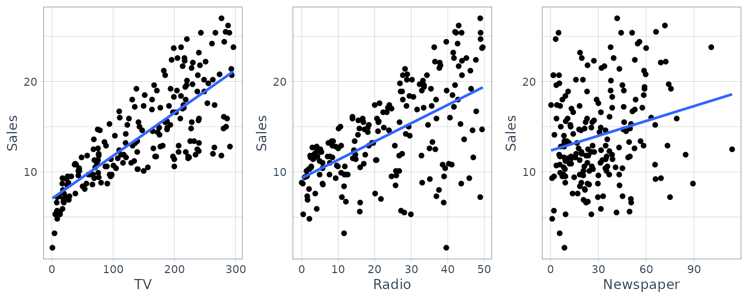
# ℹ Use `print(n = ...)` to see more rows Graphing the sales data for TV, radio, and newspapar media in the Advertising data:
plot_grid(
  ggplot(
    Advertising,
    aes(x = TV, y = sales)
  ) +
    geom_point() +
    geom_smooth(method = lm, se = FALSE) +
    xlab("TV") +
    ylab("Sales") +
    theme_tq(),
  ggplot(
    Advertising,
    aes(x = radio, y = sales)
  ) +
    xlab("Radio") +
    ylab("Sales") +
    geom_point() +
    geom_smooth(method = lm, se = FALSE) +
    theme_tq(),
  ggplot(
    Advertising,
    aes(x = newspaper, y = sales)
  ) +
    geom_point() +
    geom_smooth(method = lm, se = FALSE) +
    xlab("Newspaper") +
    ylab("Sales") +
    theme_tq(),
  ncol = 3
)
Generally, we observe a quantitative response \(Y\) and \(p\) different predictors and assume a relationship between them:
\[\begin{aligned} Y &= f(\textbf{X}) + e\\ X &= \begin{bmatrix} X_{1}\\ \ \ \vdots\\ X_{p} \end{bmatrix} \end{aligned}\]Here are a few important questions:
- Is there a relationship between advertising budget and sales?
- How strong is the relationship between adveritisng budget and sales?
- Which media are associated with sales?
- How large is the association between each medium and sales?
- How accurately can we predict future sales?
- Is the relationship linear?
- Is there synergy among the advertising media?
- For example spending $50k on TV and $50k on radio might bring higher sales than allocating $100k to either TV or radio individually.
Simple Linear Regression
For a simple regression:
\[\begin{aligned} y &= \beta_{0} + \beta_{1}x + e\\ \hat{y} &= \hat{\beta}_{0} + \hat{\beta}_{1}x \end{aligned}\]An example would be the sales example:
\[\begin{aligned} \hat{\text{sales}} &= \hat{\beta}_{0} + \hat{\beta}_{1}\times \text{TV} \end{aligned}\]And the residual sum of squares (RSS):
\[\begin{aligned} \text{RSS} &= e_{1}^{2} + \cdots + e_{n}^{2}\\ &= \sum_{i=1}^{n}(y_{i}- \hat{y}_{i})^{2} \end{aligned}\]The OLS approach chooses the coefficient to minimize the RSS:
\[\begin{aligned} \hat{\beta}_{1} &= \frac{\sum_{i=1}^{n}(x_{i} - \bar{x})(y_{i} - \bar{y})}{\sum_{i=1}^{n}(x_{i}- \bar{x})^{2}}\\[5pt] \hat{\beta}_{0} &= \bar{y} - \hat{\beta}_{1}\bar{x} \end{aligned}\]Standard errors for the \(\mu\) and the coefficients:
\[\begin{aligned} \text{var}(\hat{\mu}) &= \text{SE}(\hat{\mu})^{2}\\ &= \frac{\sigma^{2}}{n}\\[5pt] \text{SE}(\hat{\beta}_{0})^{2} &= \sigma^{2}\Bigg(\frac{1}{n} + \frac{\bar{x}^{2}}{\sum_{i=1}^{n}(x_{i} - \bar{x})^{2}}\Bigg)\\[5pt] \text{SE}(\hat{\beta}_{1})^{2} &= \frac{\sigma^{2}}{\sum_{i=1}^{n}(x_{i} - \bar{x})^{2}} \end{aligned}\]The standard error for the coefficients will be smaller when the \(x_{i}\) are more spread out.
In general, \(\sigma^{2}\) is not known and estimated from the data known as the residual standard error (RSE):
\[\begin{aligned} \hat{\sigma} &= \sqrt{\frac{RSS}{n-2}}\\ &= \text{RSE} \end{aligned}\]A 95% confidence interval for the coefficients:
\[\begin{aligned} \hat{\beta}_{1} &\pm 1.96 \times SE(\hat{\beta}_{1})\\ \hat{\beta}_{0} &\pm 1.96 \times SE(\hat{\beta}_{0}) \end{aligned}\]In terms of hypothesis testing:
\[\begin{aligned} H_{0}:\ &\beta_{1} = 0\\ H_{1}:\ &\beta_{1} \neq 0 \end{aligned}\] \[\begin{aligned} t &= \frac{\hat{\beta}_{1} - 0}{SE(\hat{\beta}_{1})} \end{aligned}\]Assuming we know the coefficient exactly, the prediction of sales on the basis of TV advertising would still be off by about RSE \(\hat{\sigma}\).
The RSE provides an absolute measure of lack of fit of the model and in the units of \(Y\). The unitless \(R^{2}\) statistic provides an alternative measure of fit:
\[\begin{aligned} R^{2} &= \frac{\text{TSS} - \text{RSS}}{\text{TSS}}\\ &= 1 - \frac{\text{RSS}}{\text{TSS}} \end{aligned}\]In simple regression, the relationship between correlation \(r^{2}\) and \(R^{2}\):
\[\begin{aligned} R^{2} &= r^{2} \end{aligned}\]We fit a least squares model for the regression of number of units sold on TV advertising budget for the Advertising data:
fit <- lm(
  sales ~ TV,
  data = Advertising
)

> summary(fit)
Call:
lm(formula = sales ~ TV, data = Advertising)

Residuals:
    Min      1Q  Median      3Q     Max
-8.3860 -1.9545 -0.1913  2.0671  7.2124

Coefficients:
            Estimate Std. Error t value            Pr(>|t|)
(Intercept) 7.032594   0.457843   15.36 <0.0000000000000002 ***
TV          0.047537   0.002691   17.67 <0.0000000000000002 ***
---
Signif. codes:  0 ‘***’ 0.001 ‘**’ 0.01 ‘*’ 0.05 ‘.’ 0.1 ‘ ’ 1

Residual standard error: 3.259 on 198 degrees of freedom
Multiple R-squared:  0.6119,	Adjusted R-squared:  0.6099
F-statistic: 312.1 on 1 and 198 DF,  p-value: < 0.00000000000000022
Multiple Linear Regression
The multiple linear regression model takes the form:
\[\begin{aligned} Y &= \beta_{0} + \beta_{1}X_{1}+ \cdots + \beta_{p}X_{p} + e \end{aligned}\]We interpret \(\beta_{j}\) as the average effect on \(Y\) of a one unit increase in \(X_{j}\) holding all other predictors fixed. For example:
\[\begin{aligned} \text{sales} &= \beta_{0} + \beta_{1}\times \text{TV} + \beta_{2} \times \text{radio} + \beta_{3} \times \text{newspaper} + e \end{aligned}\]Given the estimates, we can make prediction using:
\[\begin{aligned} \hat{y} &= \hat{\beta}_{0} + \hat{\beta}_{1}x_{1} + \cdots + \hat{\beta}_{p}x_{p} \end{aligned}\]The estimates are calcluated by minimizing the RSS:
\[\begin{aligned} RSS &= \sum_{i=1}^{n}(y_{} - \hat{y})^{2} \end{aligned}\]But how do we interpret the coefficients? For example the coefficients for newspaper in the multiple regression model is close to 0 but not in the simple linear regression way. The correlation between radio and newspaper is 0.35. This indicates that if we spend money on radio advertising, from the correlation we would spend money on newspaper advertising as well.
Fitting the model in R:
fit <- lm(
  sales ~ TV +
    radio +
    newspaper,
  data = Advertising
)

> summary(fit)
Call:
lm(formula = sales ~ TV + radio + newspaper, data = Advertising)

Residuals:
    Min      1Q  Median      3Q     Max
-8.8277 -0.8908  0.2418  1.1893  2.8292

Coefficients:
             Estimate Std. Error t value            Pr(>|t|)
(Intercept)  2.938889   0.311908   9.422 <0.0000000000000002 ***
TV           0.045765   0.001395  32.809 <0.0000000000000002 ***
radio        0.188530   0.008611  21.893 <0.0000000000000002 ***
newspaper   -0.001037   0.005871  -0.177                0.86
---
Signif. codes:  0 ‘***’ 0.001 ‘**’ 0.01 ‘*’ 0.05 ‘.’ 0.1 ‘ ’ 1

Residual standard error: 1.686 on 196 degrees of freedom
Multiple R-squared:  0.8972,	Adjusted R-squared:  0.8956
F-statistic: 570.3 on 3 and 196 DF,  p-value: < 0.00000000000000022
And the correlation matrix in R:
> cor(
  Advertising |>
    select(-X)
)
                  TV      radio  newspaper     sales
TV        1.00000000 0.05480866 0.05664787 0.7822244
radio     0.05480866 1.00000000 0.35410375 0.5762226
newspaper 0.05664787 0.35410375 1.00000000 0.2282990
sales     0.78222442 0.57622257 0.22829903 1.0000000
Is there a Relationship Between the Response and Predictors?
Consider the following hypothesis:
\[\begin{aligned} H_{0}:\ &\beta_{1} = \beta_{2} = \cdots = \beta_{p} = 0\\ H_{a}:\ &\text{at least one }\beta_{j}\text{ is non-zero} \end{aligned}\]Computing the F-statistic:
\[\begin{aligned} F &= \frac{\frac{TSS - RSS}{p}}{\frac{RSS}{n-p-1}} \end{aligned}\]If the linear model assumption is correct, then the mean square variance within samples:
\[\begin{aligned} E\Big[\frac{RSS}{n- p - 1}\Big] &= \sigma^{2} \end{aligned}\]And if \(H_{a}\) is true, then the mean square variance between samples:
\[\begin{aligned} E\Big[\frac{TSS - RSS}{p}\Big] &> \sigma^{2} \end{aligned}\] \[\begin{aligned} F &> 1 \end{aligned}\]The reason why we couldn’t just look at whether there are any significant predictors to conclude \(H_{a}\) is because just by chance, 5% of the p-values associated with each variable will be below 0.05. The F-statistic does not suffer this problem because it adjusts for the number of predictors.
Hence, if \(H_{0}\) is true, there is only a 5% chance that the F-statistic will result in a p-value below 0.05, regardless of the number of predictors or observations.
Feature Selection
The task of determining which predictors to keep is known as variable/feature selection. The criteria to judge the quality of a model includes:
- Mallow’s \(C_{p}\)
- Akaike Information Criterion (AIC)
- Bayesian Information Criterion (BIC)
- Adjusted R^{2}
There are 3 ways to do feature selection:
- Forward Selection
- Backward Selection
- Hybrid Selection
Backward selection cannot be used if \(p > n\) and forward selection is a greedy approach that might include variables too early that become redundant. Hybrid selection remedy this.
Unfortunately tidymodels do not support stepwise regression. But the same thing could be replicated and more superior using ridge regression:
ridge_spec <- linear_reg(
  mixture = 0,
  penalty = 0
) |>
  set_mode("regression") |>
  set_engine("glmnet")
mixture = 0 indicates ridge regression while mixture = 1 indicates lasso regression.
Predictions
Prediction intervals are always wider than confidence intervals because they incorporate both the error in the estimate for \(f(X)\) (the reducible error) and the uncertainty from the difference from the population regression plane (the irreducible error).
We use a confidence interval to quantify the uncertainty surrounding the average sales over a large number of cities. On the other hand, a prediction interval are used to quantify the uncertainty surrounding sales for a particular city.
For example, given that $100k is spent on TV advertising and $20k is spent on radio advertising in each city, the 95% confidence interval is:
fit <- lm(
  sales ~ TV +
    radio,
  data = Advertising
)

> predict(
  fit,
  tibble(
    TV = 100,
    radio = 20
  ),
  interval = "confidence"
)
       fit      lwr      upr
1 11.25647 10.98525 11.52768

> predict(
  fit,
  tibble(
    TV = 100,
    radio = 20
  ),
  interval = "prediction"
)
       fit      lwr      upr
1 11.25647 7.929616 14.58332
Qualitative Predictors
Let’s start with predictors with only two levels. For example we wish to investigate differences in credit card balance for people who own a house and those who don’t. We create an indicator or dummy variable (one-hot encoding) that takes on two differen values:
\[\begin{aligned} x_{i} &= \begin{cases} 1 & \text{if ith person owns a house}\\ 0 & \text{if ith person does not own a house} \end{cases} \end{aligned}\]This results in the model:
\[\begin{aligned} y_{i} &= \beta_{0} + \beta_{1}x_{i} + e_{i}\\ &= \begin{cases} \beta_{0} + \beta_{1} + e_{i} & \text{if ith person owns a house}\\ \beta_{0} + e_{i} & \text{if ith person does not own a house} \end{cases} \end{aligned}\]\(\beta_{0}\) can be interpreted as the average credit card balance among those who do not own a house, and \(\beta_{1}\) is the average difference in credit card balance between owners and non-owners.
If we use the following encoding:
\[\begin{aligned} x_{i} &= \begin{cases} 1 & \text{if ith person owns a house}\\ -1 & \text{if ith person does not own a house} \end{cases} \end{aligned}\]Then:
\[\begin{aligned} y_{i} &= \beta_{0} + \beta_{1}x_{i} + e_{i}\\ &= \begin{cases} \beta_{0} + \beta_{1} + e_{i} & \text{if ith person owns a house}\\ \beta_{0} - \beta_{1} + e_{i} & \text{if ith person does not own a house} \end{cases} \end{aligned}\]Now \(\beta_{0}\) can be interpreted as the overall average credit card balance, and \(\beta_{1}\) is the amount by which owners and non-owners that are above and below the average.
When a qualitative predictor has more than two levels, then additional dummy variables need to be created. For example, for the region variable with 3 levels, we create two dummy variables:
\[\begin{aligned} x_{i1} &= \begin{cases} 1 & \text{if ith person is from the South}\\ 0 & \text{if ith person is not from the South} \end{cases}\\ x_{i2} &= \begin{cases} 1 & \text{if ith person is from the West}\\ 0 & \text{if ith person is not from the West} \end{cases} \end{aligned}\]Then:
\[\begin{aligned} y_{i} &= \beta_{0} + \beta_{1}x_{i1} + \beta_{2}x_{i2} + e_{i}\\ &= \begin{cases} \beta_{0} + \beta_{1} + e_{i} & \text{if ith person is from the South}\\ \beta_{0} + \beta_{2} + e_{i} & \text{if ith person is from the West}\\ \beta_{0} + e_{i} & \text{if ith person is from the East} \end{cases} \end{aligned}\]Now \(\beta_{0}\) can be interpreted as the average credit card balance for individuals from the East, \(\beta_{1}\) can be interpreted as the difference in the average balance between people from the South versus the East, and \(\beta_{2}\) can be interpreted as the difference in the average balance between those from the West versus the East.
There will always be one fewer dummy variable than the number of levels. The level with no dummy variable is known as the baseline (East level in this example).
The coefficients from the 2 dummy region variables are non-significant but the F-test:
\[\begin{aligned} H_{0}:\ &\beta_{1} = \beta_{2} = 0 \end{aligned}\]Fails to reject the null hypothesis. This mean even though the coefficients levels are insignificant, there is still a relationship between balance and region (just that we cannot quantify it significantly).
Interactions
The standard linear regression assumes that the predictors and response are additive and linear. For example, our example assumed that the effect on sales of increasing one advertising medium is independent of the amount spent on the other media. For example, the linear model states that the average increase in sales associated with a one-unit increase in TV is always \(\beta_{1}\), regardless of the amount spent on radio.
One way to extend the model is to include a third predictor, called an interaction term, which is constructed by computing the product of \(X_{1}, X_{2}\):
\[\begin{aligned} Y &= \beta_{0} + \beta_{1}X_{1} + \beta_{2}X_{2}+ \beta_{3}X_{1}X_{2} + e\\ &= \beta_{0} + (\beta_{1}\beta_{3}X_{2})X_{1} + \beta_{2}X_{2} + e\\ &= \beta_{0} + \tilde{\beta}_{1}X_{1} + \beta_{2}X_{2} + e \end{aligned}\] \[\begin{aligned} \tilde{\beta}_{1} &= \beta_{1}\beta_{3}X_{2} \end{aligned}\]Since \(\tilde{\beta}_{1}\) is now a function of \(X_{2}\), the association between \(X_{1}\) and \(Y\) is no longer a constant.
For example, we fit a model with interaction term:
\[\begin{aligned} \text{sales} &= \beta_{0} + \beta_{1}\times\text{TV} + \beta_{2}\times\text{radio} + \beta_{3}\times\text{radio}\times\text{TV} + e\\ &= \beta_{0} + (\beta_{1} + \beta_{3} \times \text{radio})\times\text{TV} + \beta_{2}\times\text{radio} + e\\ &= \beta_{0} + \beta_{1}\times\text{TV} + (\beta_{2} + \beta_{3} \times \text{TV})\times\text{radio} + e \end{aligned}\]We can interpret \(\beta_{3}\) as the increase in the effectiveness of TV advertising associated with a one-unit increase in radio advertising or an increase in the effectiveness of radio advertising associated with a one-unit increase in TV advertising.
Fitting in R:
fit <- lm(
  sales ~ TV * radio,
  data = Advertising
)

> summary(fit)
Call:
lm(formula = sales ~ TV * radio, data = Advertising)

Residuals:
    Min      1Q  Median      3Q     Max
-6.3366 -0.4028  0.1831  0.5948  1.5246

Coefficients:
              Estimate Std. Error t value            Pr(>|t|)
(Intercept) 6.75022020 0.24787137  27.233 <0.0000000000000002 ***
TV          0.01910107 0.00150415  12.699 <0.0000000000000002 ***
radio       0.02886034 0.00890527   3.241              0.0014 **
TV:radio    0.00108649 0.00005242  20.727 <0.0000000000000002 ***
---
Signif. codes:  0 ‘***’ 0.001 ‘**’ 0.01 ‘*’ 0.05 ‘.’ 0.1 ‘ ’ 1

Residual standard error: 0.9435 on 196 degrees of freedom
Multiple R-squared:  0.9678,	Adjusted R-squared:  0.9673
F-statistic:  1963 on 3 and 196 DF,  p-value: < 0.00000000000000022
The hierarchical principle states that if we include an interaction in a model, we should also include the main effects, even if the p-values associated with their coefficients are not significant.
If one of the variable is a qualitative variable, it has a nice interpretation. Consider the credit example:
\[\begin{aligned} \text{balance}_{i} &\approx \beta_{0} + \beta_{1} \times \text{income}_{i} + \begin{cases} \beta_{2} & \text{if ith is a student}\\ 0 & \text{if ith person is not a student} \end{cases}\\ &= \beta_{1} \times \text{income}_{i} + \begin{cases} \beta_{0} + \beta_{2} & \text{if ith is a student}\\ \beta_{0} & \text{if ith person is not a student} \end{cases} \end{aligned}\]Notice that in both cases (student or not), the intercept is not the same but the slopes are the same. This same slope limitation can be addressed by adding an interaction term:
\[\begin{aligned} \text{balance}_{i} &\approx \beta_{0} + \beta_{1} \times \text{income}_{i} + \begin{cases} \beta_{2} + \beta_{3}\times\text{income}_{i} & \text{if ith is a student}\\ 0 & \text{if ith person is not a student} \end{cases}\\ &= \begin{cases} (\beta_{0} + \beta_{2}) + (\beta_{1} + \beta_{3})\times \text{income}_{i} & \text{if ith is a student}\\ \beta_{0} + \beta_{1} \times \text{income}_{i} & \text{if ith person is not a student} \end{cases} \end{aligned}\]Now we have different intercepts, and different slopes as well. This allows for the possibility that changes in income may affect the credit card balances of students and non-students differently.
NonLinear Relationships
A simple non-linear relationship is the polynomial regression. Consider the mpg dataset. We can fit the following quadratic model:
\[\begin{aligned} \text{mpg} &= \beta_{0} + \beta_{1} \times \text{horsepower} + \beta_{2}\times\text{horsepower}^{2} + e \end{aligned}\]This is still a linear model in the sense that:
\[\begin{aligned} X_{1} &= \text{horsepower}\\ X_{2} &= \text{horsepower}^{2} \end{aligned}\]So we can use standard OLS to estimate the coefficients.
fit <- lm(
  mpg ~ horsepower + I(horsepower^2),
  data = Auto
)

> summary(fit)
Call:
lm(formula = mpg ~ horsepower + I(horsepower^2), data = Auto)

Residuals:
     Min       1Q   Median       3Q      Max
-14.7135  -2.5943  -0.0859   2.2868  15.8961

Coefficients:
                  Estimate Std. Error t value Pr(>|t|)
(Intercept)     56.9000997  1.8004268   31.60   <2e-16 ***
horsepower      -0.4661896  0.0311246  -14.98   <2e-16 ***
I(horsepower^2)  0.0012305  0.0001221   10.08   <2e-16 ***
---
Signif. codes:  0 ‘***’ 0.001 ‘**’ 0.01 ‘*’ 0.05 ‘.’ 0.1 ‘ ’ 1

Residual standard error: 4.374 on 389 degrees of freedom
  (5 observations deleted due to missingness)
Multiple R-squared:  0.6876,	Adjusted R-squared:  0.686
F-statistic:   428 on 2 and 389 DF,  p-value: < 2.2e-16

pred <- tibble(
  x = Auto$horsepower,
  y = predict(
    fit,
    tibble(horsepower = Auto$horsepower))
)

Auto |>
  ggplot(aes(x = horsepower, y = mpg)) +
  geom_point() +
  stat_smooth(
    method = "lm",
    col = "red",
    se = FALSE
  ) +
  geom_line(
    aes(x = x, y = y),
    col = "blue",
    data = pred
  ) +
  theme_tq()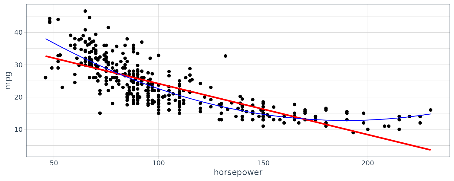
Potential Problems
Non-Linearity of the Data
Residual plots are a useful graphical tool for identifying non-linearity. To illustrate this, we compare the residual plots of a linear and quadratic curve:
fit1 <- lm(
  mpg ~ horsepower,
  data = Auto
)
fit2 <- lm(
  mpg ~ horsepower + I(horsepower^2),
  data = Auto
)

Auto$residuals1 <- fit1$residuals
Auto$residuals2 <- fit2$residuals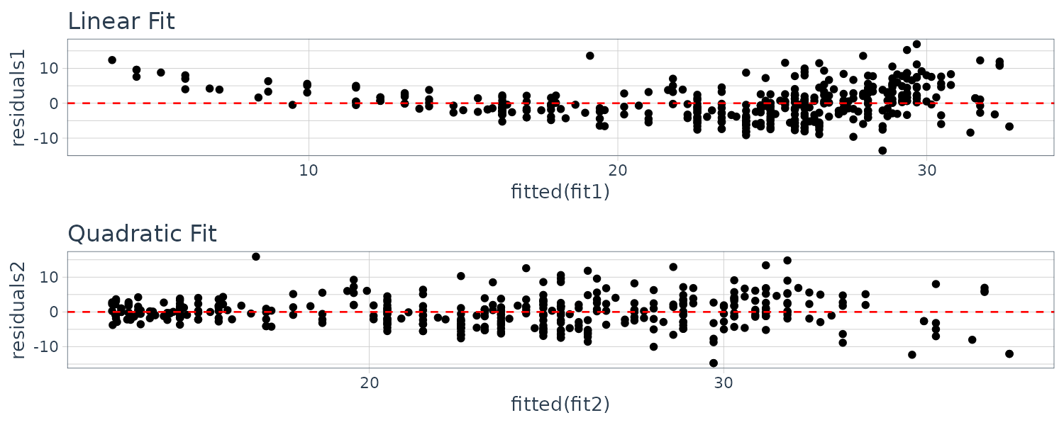
The quadratic residuals indicate a better fit.
Simple non-linear transformation of the predictors, such as \(\mathrm{log}(X), \sqrt{X}, X^{2}\) might help.
2. Correlation of Error Terms
The standard errors computed in OLS are based on the assumption of uncorrelated error terms. If there is correlation among the error terms, then the estimated standard errors will tend to underestimate the true standard errors. This will result in confidence and prediction intervals that will be narrower.
A simple example to this is to double the data by having identical pairs of observations. The resulting confidence intervals would be narrower by a factor of \(\sqrt{2}\).
3. Non-constant Variance of Error Terms
One can identify non-constant variances in the errors, or heteroscedasticity, from the presence of a funnel shape in the residual plot. One possible solution is to transform the response \(Y\) using a concave function such as \(\log Y, \sqrt{Y}\). Such a transformation results in a greater amount of shrinkage of the larger response value, leading to a reduction in heteroscedasticity.
Another solution is to use weighted least squares, with weights proportional to the inverse variances \(w_{i} = n_{i}\). \(n_{i}\) is the number of ith response raw observations and the average has variance \(\sigma^{2} = \frac{\sigma^{2}}{n_{i}}\). Larger number of observations have lower variance.
4. Outliers
An outlier is a point for which \(y_{i}\) is far from the value predicted by the outlier model. Residual plots can be used to identify outliers.
In practice, it can be difficult to decide how large a residual needs to be before we consider the point to be an outlier. To address this problem, instead of plotting the residuals, we can plot the studentized residuals, computed by dividing each residual ei by its estimated standard studentized error. Observations whose studentized residuals are greater than 3 in absolute value are possible outliers.
If we believe that an outlier has occurred due to an error in data collection or recording, then one solution is to simply remove the observation. However, care should be taken, since an outlier may instead indicate a deficiency with the model, such as a missing predictor.
5. High Leverage Points
Observations with high leverage have an unusual value for \(x_{i}\). Removing the high leverage observation has a much more substantial impact on the least squares line than removing the outlier. In fact, high leverage observations tend to have a sizable impact on the estimated regression line. It is cause for concern if the least squares line is heavily affected by just a couple of observations
In a simple linear regression, high leverage observations are fairly easy to identify, since we can simply look for observations for which the predictor value is outside of the normal range of the observations. But in a multiple linear regression with many predictors, it is possible to have an observation that is well within the range of each individual predictor’s values, but that is unusual in terms of the full set of predictors.
In order to quantify an observation’s leverage, we compute the leverage statistic. A large value of this statistic indicates an observation with high leverage. For a simple linear regression:
\[\begin{aligned} h_{i} &= \frac{1}{n} + \frac{(x_{i} - \bar{x})^{2}}{\sum_{j=1}^{n}(x_{j} - \bar{x})^{2}} \end{aligned}\]In other words, \(h_{i}\) increases with the distance of \(x_{i}\) from \(\bar{x}\). There is a simple extension of \(h_{i}\) to multiple predictors which we would not show here.
The leverage statistic \(h_{i}\) is always between \(\frac{1}{n}\) and 1, and the average leverage for all the observations is always equal to \(\frac{p+1}{n}\). So if a given observation has a leverage statistic that greatly exceeds \(\frac{p+1}{n}\), then we may suspect that the corresponding point has high leverage.
High leverage points can be calculated in R via the hatvalues() function:
hatvalues(fit)
which.max(hatvalues(lm.fit))
6. Collinearity
Collinearity refers to the situation in which two or more predictor variables collinearity are closely related to one another. The presence of collinearity can pose problems in the regression context, since it can be difficult to separate out the individual effects of collinear variables on the response. This results in a great deal of uncertainty in the coefficient estimates.
Since collinearity reduces the accuracy of the estimates of the regression coefficients, it causes the standard error for \(\hat{\beta}_{j}\) to grow. As a result, we may fail to reject \(H_{0}: \beta_{j} = 0\). This means that the power of the hypothesis test is reduced by collinearity.
A simple way to detect collinearity is to look at the correlation matrix of the predictors. An element of this matrix that is large in absolute value indicates a pair of highly correlated variables, and therefore a collinearity problem in the data. Unfortunately, not all collinearity problems can be detected by inspection of the correlation matrix: it is possible for collinearity to exist between three or more variables even if no pair of variables has a particularly high correlation. We call this situation multicollinearity.
Instead of inspecting the correlation matrix, a better way to assess multicollinearity is to compute the variance inflation factor (VIF). The VIF is variance the ratio of the variance of \(\hat{\beta}_{j}\) when fitting the full model divided by the inflation variance of \(\hat{\beta}_{j}\) if fit on its own. The smallest possible value for VIF is 1, factor which indicates the complete absence of collinearity. As a rule of thumb, a VIF value that exceeds 5 or 10 indicates a problematic amount of collinearity.
\[\begin{aligned} VIF(\hat{\beta}_{j}) &= \frac{1}{1 - R^{2}_{X_{j}\mid X_{-j}}} \end{aligned}\]Where \(R_{X_{j}\mid X_{-j}}\) is the \(R^{2}\) from a regression of \(X_{j}\) onto all of the other predictors.
When faced with the problem of collinearity, there are two simple solutions. The first is to drop one of the problematic variables from the regression. This can usually be done without much compromise to the regression fit, since the presence of collinearity implies that the information that this variable provides about the response is redundant in the presence of the other variables. The second solution is to combine the collinear variables together into a single predictor. For instance, we might take the average of standardized versions of the correlated variables.
Lab: Simple Linear Regression
Using the Boston dataset in ISLR2 library which records medv (median house value) for 506 census tracts in Boston. Predictor lstat is the percent of households with low socioeconomic status:
library(ISLR2)
lm.fit <- lm(
  medv ~ lstat,
  data = Boston
)

> summary(lm.fit)
Call:
lm(formula = medv ~ lstat, data = Boston)

Residuals:
    Min      1Q  Median      3Q     Max
-15.168  -3.990  -1.318   2.034  24.500

Coefficients:
            Estimate Std. Error t value            Pr(>|t|)
(Intercept) 34.55384    0.56263   61.41 <0.0000000000000002 ***
lstat       -0.95005    0.03873  -24.53 <0.0000000000000002 ***
---
Signif. codes:  0 ‘***’ 0.001 ‘**’ 0.01 ‘*’ 0.05 ‘.’ 0.1 ‘ ’ 1

Residual standard error: 6.216 on 504 degrees of freedom
Multiple R-squared:  0.5441,	Adjusted R-squared:  0.5432
F-statistic: 601.6 on 1 and 504 DF,  p-value: < 0.00000000000000022
We can use the names() function to find what information is stored in lm.fit:
> names(lm.fit)
 [1] "coefficients"  "residuals"     "effects"       "rank"
 [5] "fitted.values" "assign"        "qr"            "df.residual"
 [9] "xlevels"       "call"          "terms"         "model"
But it is safer to use the extractor functions like coef():
> coef(lm.fit)
(Intercept)       lstat
 34.5538409  -0.9500494
And the confidence interval for the coefficients:
> confint(lm.fit)
                2.5 %     97.5 %
(Intercept) 33.448457 35.6592247
lstat       -1.026148 -0.8739505
The predict() function can be used to produce confidence intervals and prediction intervals:
> predict(
  lm.fit, data.frame(lstat = (c(5, 10, 15))),
  interval = "confidence"
)
       fit      lwr      upr
1 29.80359 29.00741 30.59978
2 25.05335 24.47413 25.63256
3 20.30310 19.73159 20.87461

> predict(
  lm.fit, data.frame(lstat = (c(5, 10, 15))),
  interval = "prediction"
)
       fit       lwr      upr
1 29.80359 17.565675 42.04151
2 25.05335 12.827626 37.27907
3 20.30310  8.077742 32.52846
And plotting the fit:
Boston |>
  ggplot(
    aes(
      x = lstat,
      y = medv
    )
  ) +
  geom_point() +
  geom_abline(
    aes(
      intercept = coef(lm.fit)[1],
      slope = coef(lm.fit)[2],
      col = "red"
    )
  ) +
  theme_bw() +
  theme(legend.position = "none")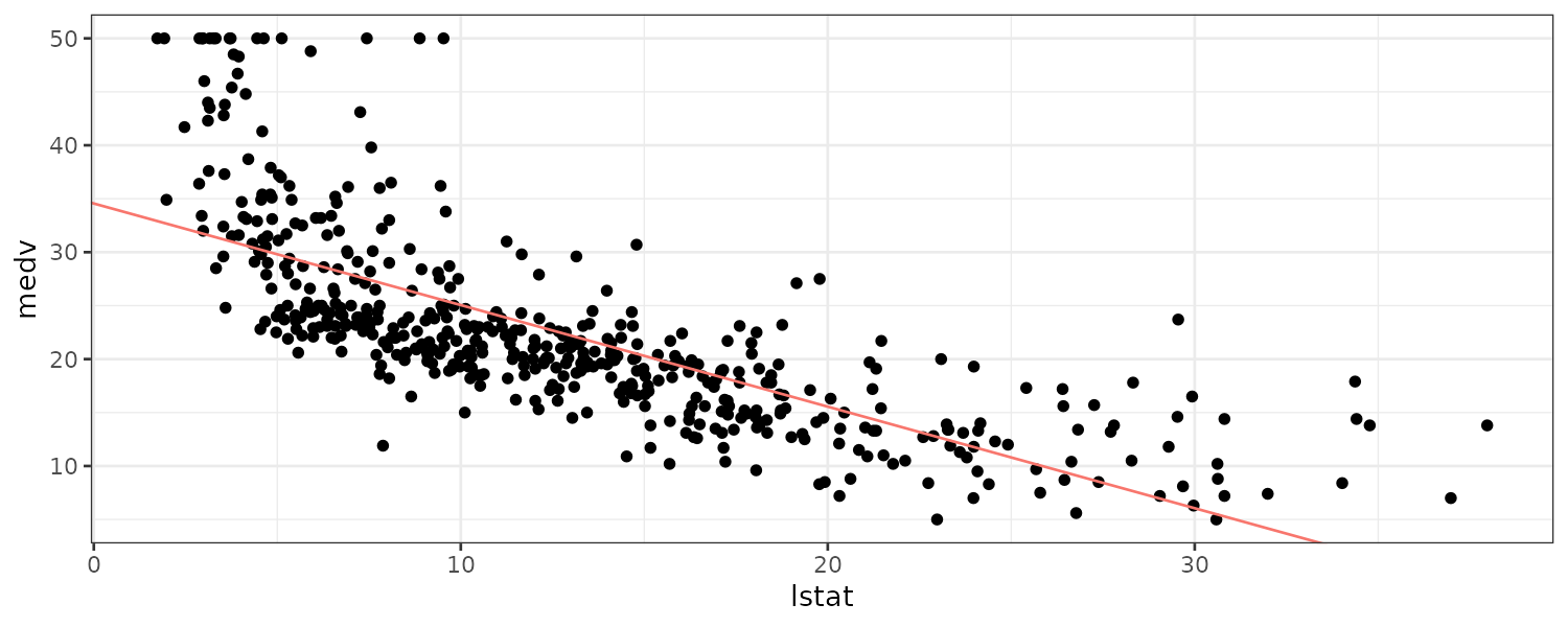
Plotting diagnostic plots:
par(mfrow = c(2, 2))
plot(lm.fit)
par(mfrow = c(1, 1)) 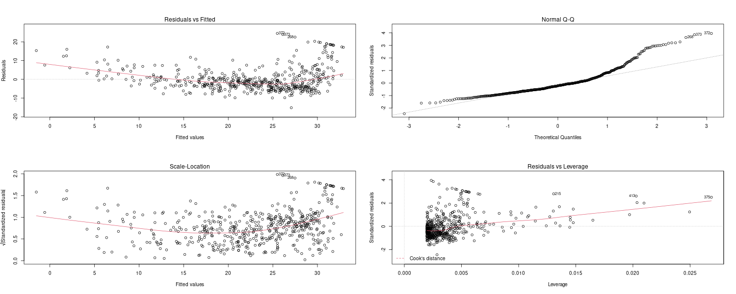
Leverage statistics can be computed for any number of predictors using the hatvalues() function:
Boston$leverage <- hatvalues(lm.fit)

> which.max(Boston$leverage)
[1] 375
Lab: Multiple Linear Regression
Fitting a multiple linear regression:
lm.fit <- lm(
  medv ~ lstat + age,
  data = Boston
)

> summary(lm.fit)
Call:
lm(formula = medv ~ lstat + age, data = Boston)

Residuals:
    Min      1Q  Median      3Q     Max
-15.981  -3.978  -1.283   1.968  23.158

Coefficients:
            Estimate Std. Error t value             Pr(>|t|)
(Intercept) 33.22276    0.73085  45.458 < 0.0000000000000002 ***
lstat       -1.03207    0.04819 -21.416 < 0.0000000000000002 ***
age          0.03454    0.01223   2.826              0.00491 **
---
Signif. codes:  0 ‘***’ 0.001 ‘**’ 0.01 ‘*’ 0.05 ‘.’ 0.1 ‘ ’ 1

Residual standard error: 6.173 on 503 degrees of freedom
Multiple R-squared:  0.5513,	Adjusted R-squared:  0.5495
F-statistic:   309 on 2 and 503 DF,  p-value: < 0.00000000000000022
Or to fit all variables:
lm.fit <- lm(
  medv ~ .,
  data = Boston
)

> summary(lm.fit)
Call:
lm(formula = medv ~ ., data = Boston)

Residuals:
     Min       1Q   Median       3Q      Max
-16.8689  -2.5782  -0.3231   1.9829  24.7183

Coefficients:
              Estimate Std. Error t value             Pr(>|t|)
(Intercept)  40.542879   4.445811   9.119 < 0.0000000000000002 ***
crim         -0.162491   0.029959  -5.424    0.000000091692872 ***
zn            0.024736   0.012667   1.953              0.05141 .
indus         0.040254   0.056014   0.719              0.47270
chas          2.545092   0.783883   3.247              0.00125 **
nox         -17.086756   3.471449  -4.922    0.000001170347450 ***
rm            2.903474   0.384844   7.545    0.000000000000221 ***
age           0.031636   0.012281   2.576              0.01029 *
dis          -1.200730   0.183538  -6.542    0.000000000152401 ***
rad           0.280870   0.060253   4.662    0.000004048005030 ***
tax          -0.011166   0.003426  -3.260              0.00119 **
ptratio      -0.802366   0.119706  -6.703    0.000000000056154 ***
lstat        -0.919290   0.056951 -16.142 < 0.0000000000000002 ***
leverage    912.248029  84.691313  10.771 < 0.0000000000000002 ***
---
Signif. codes:  0 ‘***’ 0.001 ‘**’ 0.01 ‘*’ 0.05 ‘.’ 0.1 ‘ ’ 1

Residual standard error: 4.32 on 492 degrees of freedom
Multiple R-squared:  0.785,	Adjusted R-squared:  0.7793
F-statistic: 138.2 on 13 and 492 DF,  p-value: < 0.00000000000000022
We can also retrieve the info individually from summary():
> summary(lm.fit)$r.sq
[1] 0.785007

> summary(lm.fit)$sigma
[1] 4.320425
To check the VIFs:
> car::vif(lm.fit)
    crim       zn    indus     chas      nox       rm      age      dis
1.796632 2.361124 3.995055 1.072476 4.377838 1.978089 3.233350 4.041003
     rad      tax  ptratio    lstat leverage
7.446589 9.017386 1.817027 4.474720 1.880704
We can also exclude terms via:
lm.fit1 <- lm(
  medv ~ . - age,
  data = Boston
)

lm.fit1 <- update(
  lm.fit,
  ~ . - age
)
Using interaction terms:
lm.fit <- lm(
  medv ~ lstat * age,
  data = Boston
)

> summary(lm.fit)
Call:
lm(formula = medv ~ lstat * age, data = Boston)

Residuals:
    Min      1Q  Median      3Q     Max
-15.806  -4.045  -1.333   2.085  27.552

Coefficients:
              Estimate Std. Error t value             Pr(>|t|)
(Intercept) 36.0885359  1.4698355  24.553 < 0.0000000000000002 ***
lstat       -1.3921168  0.1674555  -8.313 0.000000000000000878 ***
age         -0.0007209  0.0198792  -0.036               0.9711
lstat:age    0.0041560  0.0018518   2.244               0.0252 *
---
Signif. codes:  0 ‘***’ 0.001 ‘**’ 0.01 ‘*’ 0.05 ‘.’ 0.1 ‘ ’ 1

Residual standard error: 6.149 on 502 degrees of freedom
Multiple R-squared:  0.5557,	Adjusted R-squared:  0.5531
F-statistic: 209.3 on 3 and 502 DF,  p-value: < 0.00000000000000022
We can also fit a quadratic regression in R:
lm.fit <- lm(
  medv ~ lstat + I(lstat^2),
  data = Boston
)

> summary(lm.fit)
Call:
lm(formula = medv ~ lstat + I(lstat^2), data = Boston)

Residuals:
     Min       1Q   Median       3Q      Max
-15.2834  -3.8313  -0.5295   2.3095  25.4148

Coefficients:
             Estimate Std. Error t value            Pr(>|t|)
(Intercept) 42.862007   0.872084   49.15 <0.0000000000000002 ***
lstat       -2.332821   0.123803  -18.84 <0.0000000000000002 ***
I(lstat^2)   0.043547   0.003745   11.63 <0.0000000000000002 ***
---
Signif. codes:  0 ‘***’ 0.001 ‘**’ 0.01 ‘*’ 0.05 ‘.’ 0.1 ‘ ’ 1

Residual standard error: 5.524 on 503 degrees of freedom
Multiple R-squared:  0.6407,	Adjusted R-squared:  0.6393
F-statistic: 448.5 on 2 and 503 DF,  p-value: < 0.00000000000000022
I() is needed here because caret has a special meaining in a formula object.
We can use anova() to see whether a more complex model is statistically signifcant:
> anova(lm.fit2, lm.fit)
Analysis of Variance Table

Model 1: medv ~ lstat
Model 2: medv ~ lstat + I(lstat^2)
  Res.Df   RSS Df Sum of Sq     F                Pr(>F)
1    504 19472
2    503 15347  1    4125.1 135.2 < 0.00000000000000022 ***
---
Signif. codes:  0 ‘***’ 0.001 ‘**’ 0.01 ‘*’ 0.05 ‘.’ 0.1 ‘ ’ 1
In general, we can use the poly() function to create a polynomial fit within lm():
lm.fit <- lm(
  medv ~ poly(lstat , 5),
  data = Boston
)

> summary(lm.fit)
Call:
lm(formula = medv ~ poly(lstat, 5), data = Boston)

Residuals:
     Min       1Q   Median       3Q      Max
-13.5433  -3.1039  -0.7052   2.0844  27.1153

Coefficients:
                 Estimate Std. Error t value             Pr(>|t|)
(Intercept)       22.5328     0.2318  97.197 < 0.0000000000000002 ***
poly(lstat, 5)1 -152.4595     5.2148 -29.236 < 0.0000000000000002 ***
poly(lstat, 5)2   64.2272     5.2148  12.316 < 0.0000000000000002 ***
poly(lstat, 5)3  -27.0511     5.2148  -5.187           0.00000031 ***
poly(lstat, 5)4   25.4517     5.2148   4.881           0.00000142 ***
poly(lstat, 5)5  -19.2524     5.2148  -3.692             0.000247 ***
---
Signif. codes:  0 ‘***’ 0.001 ‘**’ 0.01 ‘*’ 0.05 ‘.’ 0.1 ‘ ’ 1

Residual standard error: 5.215 on 500 degrees of freedom
Multiple R-squared:  0.6817,	Adjusted R-squared:  0.6785
F-statistic: 214.2 on 5 and 500 DF,  p-value: < 0.00000000000000022
By default, the poly() function orthogonalizes the predictors. However, a linear model applied to the output of the poly() function will have the same fitted values as a linear model applied to the raw polynomials (although the coefficient estimates, standard errors, and p-values will differ).
In order to obtain the raw polynomials from the poly() function, the argument raw = TRUE must be used:
lm.fit <- lm(
  medv ~ poly(lstat , 5, raw = TRUE),
  data = Boston
)

> summary(lm.fit)
Call:
lm(formula = medv ~ poly(lstat, 5, raw = TRUE), data = Boston)

Residuals:
     Min       1Q   Median       3Q      Max
-13.5433  -3.1039  -0.7052   2.0844  27.1153

Coefficients:
                                Estimate   Std. Error t value             Pr(>|t|)
(Intercept)                  67.69967680   3.60429465  18.783 < 0.0000000000000002 ***
poly(lstat, 5, raw = TRUE)1 -11.99111682   1.52571799  -7.859   0.0000000000000239 ***
poly(lstat, 5, raw = TRUE)2   1.27281826   0.22316694   5.703   0.0000000201146101 ***
poly(lstat, 5, raw = TRUE)3  -0.06827384   0.01438227  -4.747   0.0000026985438437 ***
poly(lstat, 5, raw = TRUE)4   0.00172607   0.00041666   4.143   0.0000403207827613 ***
poly(lstat, 5, raw = TRUE)5  -0.00001632   0.00000442  -3.692             0.000247 ***
---
Signif. codes:  0 ‘***’ 0.001 ‘**’ 0.01 ‘*’ 0.05 ‘.’ 0.1 ‘ ’ 1

Residual standard error: 5.215 on 500 degrees of freedom
Multiple R-squared:  0.6817,	Adjusted R-squared:  0.6785
F-statistic: 214.2 on 5 and 500 DF,  p-value: < 0.00000000000000022
Lab: Qualitative Predictors
Consider the Carseats data. We will attempt to predict Sales (child car seat sales) in 400 locations based on a number of predictors:
lm.fit <- lm(
  Sales ~ . + Income:Advertising + Price:Age,
  data = Carseats
)

> summary(lm.fit)
Call:
lm(formula = Sales ~ . + Income:Advertising + Price:Age, data = Carseats)

Residuals:
    Min      1Q  Median      3Q     Max
-2.9208 -0.7503  0.0177  0.6754  3.3413

Coefficients:
                     Estimate Std. Error t value             Pr(>|t|)
(Intercept)         6.5755654  1.0087470   6.519       0.000000000222 ***
CompPrice           0.0929371  0.0041183  22.567 < 0.0000000000000002 ***
Income              0.0108940  0.0026044   4.183       0.000035665275 ***
Advertising         0.0702462  0.0226091   3.107             0.002030 **
Population          0.0001592  0.0003679   0.433             0.665330
Price              -0.1008064  0.0074399 -13.549 < 0.0000000000000002 ***
ShelveLocGood       4.8486762  0.1528378  31.724 < 0.0000000000000002 ***
ShelveLocMedium     1.9532620  0.1257682  15.531 < 0.0000000000000002 ***
Age                -0.0579466  0.0159506  -3.633             0.000318 ***
Education          -0.0208525  0.0196131  -1.063             0.288361
UrbanYes            0.1401597  0.1124019   1.247             0.213171
USYes              -0.1575571  0.1489234  -1.058             0.290729
Income:Advertising  0.0007510  0.0002784   2.698             0.007290 **
Price:Age           0.0001068  0.0001333   0.801             0.423812
---
Signif. codes:  0 ‘***’ 0.001 ‘**’ 0.01 ‘*’ 0.05 ‘.’ 0.1 ‘ ’ 1

Residual standard error: 1.011 on 386 degrees of freedom
Multiple R-squared:  0.8761,	Adjusted R-squared:  0.8719
F-statistic:   210 on 13 and 386 DF,  p-value: < 0.00000000000000022
The contrasts() function returns the coding that R uses for the dummy variables:
> contrasts(Carseats$ShelveLoc)
       Good Medium
Bad       0      0
Good      1      0
Medium    0      1
R has created a ShelveLocGood dummy variable that takes on a value of 1 if the shelving location is good, and 0 otherwise. It has also created a ShelveLocMedium dummy variable that equals 1 if the shelving location is medium, and 0 otherwise. A bad shelving location corresponds to a zero for each of the two dummy variables.
Classification
Logistic Regression
Consider the Default data set. Rather than modeling the response Y directly, logistic regression models the probability that Y belongs to a particular category.
\[\begin{aligned} P(\text{default} = \text{Yes}|\text{balance}) \end{aligned}\]Consider the logistic function, which outputs between 0 and 1 for all values of X:
\[\begin{aligned} p(X) &= \frac{e^{\beta_{0} + \beta_{1}X}}{1 + e^{\beta_{0} + \beta_{1}X}} \end{aligned}\]We can manipulate the above equation to get the odds on the LHS:
\[\begin{aligned} \frac{p(X)}{1 - p(X)} &= e^{\beta_{0} + \beta_{1}X} \end{aligned}\]The odds can take any value between 0 and \(\infty\).
For example, on average 1 in 5 people with an odds of \(\frac{1}{4}\) will default, since \(p(X) = 0.2\) implies an odds of \(\frac{0.2}{1 - 0.2} = \frac{1}{4}\). Likewise, on average nine out of every ten people with an odds of 9 will default, since \(p(X) = 0.9\) implies an odds of \(\frac{0.9}{1 - 0.9} = 9\).
Odds are traditionally used instead of probabilities in horse-racing, since they relate more naturally to the correct betting strategy.
The log-odds or logit:
\[\begin{aligned} \mathrm{log}\Big(\frac{p(X)}{1 - p(X)}\Big) &= \beta_{0} + \beta_{1}X \end{aligned}\]By increasing X one-unit changes the log-odds by \(\beta_{1}\), or the odds by \(e^{\beta_{1}}\).
To estimate the coefficients, we can use nls to fit:
\[\begin{aligned} \mathrm{log}\Big(\frac{p(X)}{1 - p(X)}\Big) &= \beta_{0} + \beta_{1}X \end{aligned}\]Or use MLE by finding the coefficients that maximize the likelihood:
\[\begin{aligned} l(\beta_{0}, \beta_{1}) &= \prod_{i:y_{i} = 1}p(x_{i})\prod_{i:y_{i} = 0}(1 - p(x_{i})) \end{aligned}\]Fitting the logistic regression in R:
fit <- glm(
  default ~ balance,
  data = Default,
  family = "binomial"
)

> summary(fit)
Call:
glm(formula = default ~ balance, family = "binomial", data = Default)

Deviance Residuals:
    Min       1Q   Median       3Q      Max
-2.2697  -0.1465  -0.0589  -0.0221   3.7589

Coefficients:
               Estimate  Std. Error z value            Pr(>|z|)
(Intercept) -10.6513306   0.3611574  -29.49 <0.0000000000000002 ***
balance       0.0054989   0.0002204   24.95 <0.0000000000000002 ***
---
Signif. codes:  0 ‘***’ 0.001 ‘**’ 0.01 ‘*’ 0.05 ‘.’ 0.1 ‘ ’ 1

(Dispersion parameter for binomial family taken to be 1)

    Null deviance: 2920.6  on 9999  degrees of freedom
Residual deviance: 1596.5  on 9998  degrees of freedom
AIC: 1600.5

Number of Fisher Scoring iterations: 8
Using the coefficient estimates from R, we predict that the default probability for an individual with a balance of $1,000 is:
\[\begin{aligned} \hat{p}(X) &= \frac{e^{\hat{\beta}_{0} + \hat{\beta}_{1}X}}{1 + e^{\hat{\beta}_{0} + \hat{\beta}_{1}X}}\\ &= \frac{e^{-10.65 + 0.0055 \times 1000}}{1 + e^{-10.65 + 0.0055 \times 1000}}\\ &= 0.00576 \end{aligned}\]And the prediction in R:
> predict(
  fit,
  tibble(
    balance = 1000
  ),
  type = "response"
)
          1
0.005752145
Or using a qualitive variable student as example:
\[\begin{aligned} P(\text{default}= \text{Yes}|\text{student} = \text{Yes}) &= \frac{e^{-3.5 + 0.4 \times 1}}{1 + e^{-3.5 + 0.4 \times 1}}\\ &= 0.0431\\ P(\text{default}= \text{Yes}|\text{student} = \text{No}) &= \frac{e^{-3.5 + 0.4 \times 0}}{1 + e^{-3.5 + 0.4 \times 0}}\\ &= 0.0292 \end{aligned}\]And in R:
> predict(
  fit,
  tibble(
    student = "Yes"
  ),
  type = "response"
)
         1
0.04313859

> predict(
  fit,
  tibble(
    student = "No"
  ),
  type = "response"
)
         1
0.02919501
Multiple Logistic Regression
When we generalize it to p predictors:
\[\begin{aligned} \textrm{log}\Big(\frac{p(X)}{1 - p(X)}\Big) &= \beta_{0} + \beta_{1}X_{1} + \cdots + \beta_{p}X_{p}\\ p(X) &= \frac{e^{\beta_{0} + \beta_{1}X_{1} + \cdots + \beta_{p}X_{p}}}{1 + e^{\beta_{0} + \beta_{1}X_{1} + \cdots + \beta_{p}X_{p}}} \end{aligned}\]Fitting the Default dataset using 3 predictors in R:
fit <- glm(
  default ~ balance + income + student,
  data = Default,
  family = "binomial"
)

> summary(fit)
Call:
glm(formula = default ~ balance + income + student, family = "binomial",
    data = Default)

Deviance Residuals:
    Min       1Q   Median       3Q      Max
-2.4691  -0.1418  -0.0557  -0.0203   3.7383

Coefficients:
                 Estimate    Std. Error z value             Pr(>|z|)
(Intercept) -10.869045196   0.492255516 -22.080 < 0.0000000000000002 ***
balance       0.005736505   0.000231895  24.738 < 0.0000000000000002 ***
income        0.000003033   0.000008203   0.370              0.71152
studentYes   -0.646775807   0.236252529  -2.738              0.00619 **
---
Signif. codes:  0 ‘***’ 0.001 ‘**’ 0.01 ‘*’ 0.05 ‘.’ 0.1 ‘ ’ 1

(Dispersion parameter for binomial family taken to be 1)

    Null deviance: 2920.6  on 9999  degrees of freedom
Residual deviance: 1571.5  on 9996  degrees of freedom
AIC: 1579.5

Number of Fisher Scoring iterations: 8
Notice that the student coefficient is now negative rather than positive in the simple linear regression case. The reason is because after adjusting for balance, student tend to have lower default rates. However, since students in general have a higher credit balance, it has a higher overall default rate.
Prediction in R:
> predict(
  fit,
  tibble(
    student = "Yes",
    balance = 1500,
    income = 40000
  ),
  type = "response"
)
         1
0.05788194 > predict(
fit,
tibble(
student = "No",
balance = 1500,
income = 40000
),
type = "response"
)
1
0.1050492 Multinomial Logistic Regression
We sometimes wish to classify a response variable that has more than two classes. We first select a single class to serve as the baseline. Say we select the kth class. Then we use the following multinomial logistic regression:
\[\begin{aligned} P(Y = k|X = x) &= \frac{e^{\beta_{k0} + \beta_{k1}x_{1} + \cdots + \beta_{kp}x_{p}}}{1 + \sum_{l=1}^{K-1}e^{\beta_{l0} + \beta_{l1}x_{1} + \cdots + \beta_{lp}x_{p}}}\\ k &= 1, \cdots, K-1\\ P(Y = K|X = x) &= \frac{1}{1 + \sum_{l=1}^{K-1}e^{\beta_{l0} + \beta_{l1}x_{1} + \cdots + \beta_{lp}x_{p}}} \end{aligned}\] \[\begin{aligned} \textrm{log}\Bigg(\frac{P(Y=k|X = x)}{P(Y= K|X=x)}\Bigg) &= \beta_{k0} + \beta_{k1}x_{1} + \cdots + \beta_{kp}x_{p} \end{aligned}\]For example, if we are classifying emergency room visits into 3 categories of stroke, drug overdose, and epileptic seizure. If \(X_{j}\) increases by one unit, then:
\[\begin{aligned} \frac{P(Y = \text{stroke}|X = x)}{P(Y = \text{epileptic seizure}|X = x)} \end{aligned}\]Increases by \(e^{\beta_{strokej}}\).
There is an alternative coding for multinomial logistic regression known as softmax coding. Rather than selecting a baseline class, we treat all K classes the same:
\[\begin{aligned} P(Y = k|X = x) &= \frac{e^{\beta_{k0} + \beta_{k1}x_{1} + \cdots + \beta_{kp}x_{p}}}{1 + \sum_{l=1}^{K}e^{\beta_{l0} + \beta_{l1}x_{1} + \cdots + \beta_{lp}x_{p}}}\\ k &= 1, \cdots, K\\ \end{aligned}\]Thus, rather than estimating coefficients for K − 1 classes, we actually estimate coefficients for all K classes. The log odds ratio between kth and Kth classes would then be:
\[\begin{aligned} \textrm{log}\Bigg(\frac{P(Y=k|X = x)}{P(Y= K|X=x)}\Bigg) &= (\beta_{k0} - \beta_{K0}) + (\beta_{k1} - \beta_{K1})x_{1} + \cdots + (\beta_{kp}-\beta_{Kp})x_{p} \end{aligned}\]Generative Models for Classification
An alternative approach to directly modeling \(P(Y= k \mid X = x)\) is to model the distbution of the predictors \(X\) separately in each of the response classes, and use Bayes’ theorem to get \(P(Y= k \mid X = x)\).
Let \(P(k)\) represent the proir probability that a random chosen observation comes from the kth class. Let \(P(X\mid Y = k)\) denote the density function of \(X\) for an observation that comes from the kth class. Then Bayes’ theorem states that:
\[\begin{aligned} P(Y = k | X = x) &= \frac{P(Y=k)P(X|Y=k)}{\sum_{l=1}^{K}P(Y=l)P(X|Y = l)} \end{aligned}\]We will discuss three classifiers that use different estimates of \(P(X\mid Y=k)\) to approximate the Bayes classifier: linear discriminant analysis, quadratic discriminant analysis, and naive Bayes.
Linear Discriminant Analysis
We first touch on \(p = 1\). Next we assume that \(P(X\mid Y = k)\) is normal:
\[\begin{aligned} P(X|Y = k) &= \frac{1}{\sqrt{2\pi}\sigma_{k}}e^{-\frac{1}{2\sigma_{k}}(x - \mu_{k})^{2}} \end{aligned}\]If we assume the variance is the same across all K classes, then the posterior probability is:
\[\begin{aligned} P(Y =k|X) &= \frac{P(Y = k)\frac{1}{\sqrt{2\pi}\sigma}e^{-\frac{1}{2\sigma}(x - \mu_{k})^{2}}}{\sum_{l=1}^{K}P(Y = l)\frac{1}{\sqrt{2\pi}\sigma}e^{-\frac{1}{2\sigma}(x - \mu_{l})^{2}}} \end{aligned}\]The Bayes classifier assigns the observation to the class for which the posterior probability is the highest.
We can show that this is equivalent to assigning the observation to the class for which the below is max:
\[\begin{aligned} \delta_{k}(x) = x\frac{\mu_{k}}{\sigma^{2}} - \frac{\mu_{k}^{2}}{2\sigma^{2}} + \log(P(y = k)) \end{aligned}\]First we remove the multiplicative constant which doesn’t depend on \(k\) and take a log:
\[\begin{aligned} \ln\Big(P(Y=k)e^{-\frac{1}{2\sigma}(x - \mu_{k})^{2}}\Big) &= \ln\Big(P(Y=k)\Big)- \frac{1}{2\sigma}(x - \mu_{k})^{2}\\ &= \ln\Big(P(Y=k)\Big)- \frac{1}{2\sigma}(x^{2} - 2\mu_{k}x + \mu_{k}^{2})\\ &= \ln\Big(P(Y=k)\Big)- \frac{x^{2}}{2\sigma^{2}} + \frac{2\mu_{k}x}{2\sigma^{2}} - \frac{\mu_{k}^{2}}{2\sigma^{2}} \end{aligned}\]We can remove constant \(\frac{x^{2}}{2\sigma^{2}}\) to get:
\[\begin{aligned} x\frac{\mu_{k}}{\sigma^{2}} - \frac{\mu_{k}^{2}}{2\sigma^{2}} + \ln\Big(P(y = k)\Big) \end{aligned}\]And the decison boundary is when \(\delta_{1}(x) = \delta_{2}(x)\):
\[\begin{aligned} x &= \frac{\mu_{1}^{2} - \mu_{2}^{2}}{2(\mu_{1} - \mu_{2})}\\[5pt] &= \frac{\mu_{1} + \mu_{2}}{2} \end{aligned}\]The LDA method approximates the Bayes classifier by plugging estimates for the prior probability and mean for each class, and the varaince into the posterior probability formula:
\[\begin{aligned} \hat{\mu}_{k} &= \frac{1}{n_{k}}\sum_{i:y_{i} = k}x_{i}\\ \hat{\sigma}^{2} &= \frac{1}{n - K}\sum_{k=1}^{K}\sum_{i:y_{i} = k}(x_{i} - \hat{\mu}_{k})^{2} \end{aligned}\]To extend the LDA classifier to the case of multiple predictors, we first assume that:
\[\begin{aligned} \boldsymbol{X} = \begin{bmatrix} X_{1}\\ \vdots\\ x_{p} \end{bmatrix} \end{aligned}\]Is drawn from a multivariate Gaussian distribution. The multivariate Gaussian distribution assumes that each individual predictor follows a one-dimensional normal distribution, with some correlation between each pair of predictors.
The multivariate Gaussian density is defined as:
\[\begin{aligned} p(\boldsymbol{x}) &= \frac{1}{(2\pi)^{\frac{p}{2}}|\boldsymbol{\Sigma}^{\frac{1}{2}}}e^{-\frac{1}{2}(\boldsymbol{x} - \boldsymbol{\mu})^{T}\boldsymbol{\Sigma}^{-1}(\boldsymbol{x} - \boldsymbol{\mu})} \end{aligned}\]Finally, the Bayes classifier assigns an observation \(\boldsymbol{x}\) to the class for which the \(\delta_{k}\) is the largest:
\[\begin{aligned} \delta_{k}(\boldsymbol{x}) &= \boldsymbol{x}^{T}\boldsymbol{\Sigma}^{-1}\boldsymbol{\mu}_{k} - \frac{1}{2}\boldsymbol{\mu}_{k}^{T}\boldsymbol{\Sigma}^{-1}\boldsymbol{\mu}_{k} + \log\Big(P(Y = k)\Big) \end{aligned}\]We expect LDA to outperform logistic regression when the normality assumption (approximately) holds, and we expect logistic regression to perform better when it does not.
Quadratic Discriminant Analysis
Like LDA, the QDA classifier results from assuming that the observations discriminant from each class are drawn from a Gaussian distribution, and plugging estimates for the parameters into Bayes’ theorem in order to perform prediction.
However, unlike LDA, QDA assumes that each class has its own covariance matrix. That is, it assumes that an observation from the kth class is of the form. Under this assumption, the Bayes classifier assigns an observation to the class for which:
\[\begin{aligned} \delta_{k}(\boldsymbol{x}) &= -\frac{1}{2}(\textbf{x} - \boldsymbol{\mu}_{k})^{T}\boldsymbol{\Sigma}_{k}^{-1}(\textbf{x} - \boldsymbol{\mu}_{k}) - \frac{1}{2}\log|\boldsymbol{\Sigma_{k}}| + \log(P(Y = k))\\ &= -\frac{1}{2}\mathrm{x}^{T}\boldsymbol{\Sigma}_{k}^{-1}\mathbf{x} + \mathrm{x}^{T}\boldsymbol{\Sigma}_{k}^{-1}\boldsymbol{\mu}_{k} - \frac{1}{2}\boldsymbol{\mu}_{k}\boldsymbol{\Sigma}_{k}^{-1}\boldsymbol{\mu}_{k} - \frac{1}{2}\log|\boldsymbol{\Sigma}_{k}| + \log(P(Y= k)) \end{aligned}\]When there are p predictors, then estimating a covariance matrix requires esti mating \(\frac{p(p+1)}{2}\) parameters. QDA estimates a separate covariance matrix for each class, for a total of \(\frac{Kp(p+1)}{2}\) parameters.
By instead assuming that the K classes share a common covariance matrix, the LDA model becomes linear in x, which means there are Kp linear coefficients to estimate. Consequently, LDA is a much less flexible classifier than QDA, and so has substantially lower variance. This can potentially lead to improved prediction performance. But there is a trade-off: if LDA’s assumption that the K classes share a common covariance matrix is badly off, then LDA can suffer from high bias. Roughly speaking, LDA tends to be a better betthan QDA if there are relatively few training observations and so reducing variance is crucial.
Naive Bayes
In general, estimating a p-dimensional density function is challenging. In LDA, we make a very strong assumption that greatly simplifies the task: we assume that \(P(X|Y = k)\) is the density function for a multivariate normal random variable with class-specific mean \(\mu_{k}\), and shared covariance matrix \(\boldsymbol{\Sigma}\).
By contrast, in QDA, we assume that \(P(X\mid Y = k)\) is the density function for a multivariate normal random variable with class-specific mean \(\mu_{k}\), and class-specific covariance matrix \(\boldsymbol{\Sigma}_{k}\).
By making these very strong assumptions, we are able to replace the very challenging problem of estimating K p-dimensional density functions with the much simpler problem of estimating K p-dimensional mean vectors and one (in the case of LDA) or K (in the case of QDA) (p x p)-dimensional covariance matrices.
The naive Bayes classifier assumes within the kth class, the p predictors are independent:
\[\begin{aligned} P(\boldsymbol{x}|Y=k) &= P(X_{1} = x_{1}|Y=k)\times P(X_{2} = x_{2}|Y=k) \times \cdots \times P(X_{p} = x_{p}|Y=k) \end{aligned}\]The naive Bayes assumption introduces some bias, but reduces variance, leading to a classifier that works quite well in practice as a result of the bias-variance trade-off.
And for the posterior probability:
\[\begin{aligned} P(Y = k | X = \mathrm{x}) &= \frac{P(Y = k)\times P(X_{1} = x_{1}|Y=k)\times P(X_{2} = x_{2}|Y=k) \times \cdots \times P(X_{p} = x_{p}|Y=k)}{\sum_{l=1}^{K}P(Y = l) \times P(X_{1} = x_{1}|Y=l)\times P(X_{2} = x_{2}|Y=l) \times \cdots \times P(X_{p} = x_{p}|Y=l)} \end{aligned}\] \[\begin{aligned} k &= 1, \cdots, K \end{aligned}\]If \(X_{j}\) is quantitative, then we can assume that \(X_{j} \mid Y = k \sim N(\mu_{jk} , \sigma_{jk})\). In other words, we assume that within each class, the jth predictor is drawn from a (univariate) normal distribution. While this may sound a bit like QDA, there is one key difference, in that here we are assuming that the predictors are independent; this amounts to QDA with an additional assumption that the class-specific covariance matrix is diagonal.
| Another option is to use a non-parametric estimate for $$P(X_{j} | Y = k)\(. A very simple way to do this is by making a histogram for the observations of the jth predictor within each class. Then we can estimate\)P(X_{j} | Y = k)\(as the fraction of the training observations in the kth class that belong to the same histogram bin as\)x_{j}$$. Alternatively, we can use a kernel density estimator, which is kernel essentially a smoothed version of a histogram. |
If \(X_{j}\) is qualitative, then we can simply count the proportion of training observations for the jth predictor corresponding to each class. For instance, suppose that \(X_{j} \in \{1, 2, 3\}\), and we have 100 observations in the kth class. Suppose that the jth predictor takes on values of 1, 2, and 3 in 32, 55, and 13 of those observations, respectively. Then:
\[\begin{aligned} \hat{P}(X_{j} = x_{j} | Y = k) &= \begin{cases} 0.32 & x_{j} = 1\\ 0.55 & x_{j} = 2\\ 0.13 & x_{j} = 3 \end{cases} \end{aligned}\]See Also
References
James G, Witten D., Hastie T. Tibshirani R. (2021) An Introduction to Statistical Learning
