Time Series Analysis for the State-Space Model with R/Stan
Read PostIn this post, we will cover Hagiwara J. (2021) Time Series Analysis for the State-Space Model with R/Stan.
Contents:
Fundamentals of Probability and Statistics
Mean and Variance
The mean value (or expected value) and variance for the random variable X is defined as:
\[\begin{aligned} E[X] &= \int x p(x)\ dx \end{aligned}\] \[\begin{aligned} \text{var}(X) &= E[(X - E[X])^{2}]\\ &= \int (x - E[X])^{2}p(x)\ dx \end{aligned}\]Let a and b be constants and X and Y be random variables. The following transformation relations hold for the mean and variance:
\[\begin{aligned} E[aX + b] &= aE[X] + b\\ E[X + Y]&= E[X] + E[Y] \end{aligned}\] \[\begin{aligned} E[X + Y]&= E[X] + E[Y] \end{aligned}\] \[\begin{aligned} \text{var}(X + Y) &= \text{var}(X) + \text{var}(Y) + 2E\Big[(X - E[X])(Y - E[Y])\Big] \end{aligned}\]Relation Among Multiple Random Variables
When there are multiple random variables, the probability that they will coincide is referred to as the joint probability. The probability distribution for the joint probability is referred to as the joint distribution. Let X and Y be the random variables; their joint distribution is denoted as:
\[\begin{aligned} p(x, y) \end{aligned}\]When there are multiple random variables, the probability of only a specific random variable is referred to as the marginal probability. The probability distribution of the marginal probability is referred to as the marginal distribution:
\[\begin{aligned} p(x) &= \int p(x, y)\ dy\\ p(y) &= \int p(x, y)\ dx \end{aligned}\]Regarding the conditional distribution, the relation below holds as a result of the product rule of probability:
\[\begin{aligned} p(x | y)p(y) &= p(x, y)\\ & = p(y |x)p(x) \end{aligned}\]And from the product rule of probability, Bayes’ Theorem:
\[\begin{aligned} p(x |y) &= \frac{p(y | x)p(x)}{p(y)}\\[10pt] p(y |x) &= \frac{p(x | y)p(y)}{p(x)} \end{aligned}\]Finally, when the joint distribution can be decomposed into a simple product of each marginal distribution, the random variables are said to be independent:
\[\begin{aligned} p(x, y) &= p(x)p(y) \end{aligned}\]Stochastic Process
A stochastic process is a series of random variables, which exactly corresponds to stochastically interpreted time series data. For a sequence, to express a time point t, a subscript is assigned to the random variable and its realizations such as \(Y_{t}\) and \(y_{t}\), respectively.
Covariance and Correlation
The covariance is defined as:
\[\begin{aligned} \text{cov}(X, Y) &= E\Big[(X - E[X])(Y - E[Y])\Big] \end{aligned}\]The autocovariance of stochastic process \(X_{t}\) is defined as:
\[\begin{aligned} \text{cov}(X_{t}, X_{t-k}) &= E\Big[(X_{t} - E[X])(X_{t-k} - E[X_{t-k}])\Big] \end{aligned}\]Stationary and Nonstationary Processes
Stationarity means that a stochastic feature does not change even if time changes. In more detail, when the probability distribution for a stochastic process is invariant independently of time point t, its stochastic process is referred to as strictly stationary.
On the contrary, when mean, variance, autocovariance, and the autocorrelation coefficient for a stochastic process are invariant independently of time point t, the stochastic process is referred to as weakly stationary.
Maximum Likelihood Estimation and Bayesian Estimation
We have implicitly assumed so far that the parameter \(\boldsymbol{\theta}\) in a probability distribution is known. The parameter is sometimes known but is generally unknown and must be specified by some means for analysis.
The likelihood of the entire stochastic process \(Y_{t}\) is expressed by:
\[\begin{aligned} p(y_{1}, y_{2}, \cdots, y_{T}; \boldsymbol{\theta}) \end{aligned}\]The likelihood is a single numerical indicator of how an assumed probability distribution fits the realizations. The natural logarithm of the likelihood is referred to as the log-likelihood as:
\[\begin{aligned} l(\boldsymbol{\theta}) &= \log p(y_{1}, \cdots, y_{T};\boldsymbol{\theta}) \end{aligned}\]The maximum likelihood method specifies the parameter \(\boldsymbol{\theta}\) where the likelihood is maximized. Function log() is a monotonically increasing function with the result that the maximization of likelihood has the same meaning as that of log-likelihood.
Let \(\hat{\boldsymbol{\theta}}\) be the estimator for parameters. The maximum likelihood estimation is expressed as:
\[\begin{aligned} \hat{\boldsymbol{\theta}} &= \text{argmax}_{\boldsymbol{\theta}}\ l(\boldsymbol{\theta}) \end{aligned}\]In the above description, the parameter is not considered to be a random variable. The frequentists generally take such a viewpoint, and parameter specification through maximum likelihood estimation is one approach in frequentism.
On the other hand, there is a means of considering parameter as a random variable. Bayesians generally take this viewpoint, and a parameter is estimated through Bayesian estimation based on Bayes’ theorem under Bayesianism.
Frequency Spectrum
The frequency spectrum can be derived by converting data in the time domain to the frequency domain; it is useful for confirming periodicity. The representations in the time and frequency domains have a paired relation.
In general, any periodic time series data \(y_{t}\) can be considered as the sum of trigonometric functions with various periods. This is known as Fourier series expansion
Fourier series can be expressed using sine and cosine functions, and more briefly using complex values. Specifically, the Fourier series expansion of observations \(y_{t}\) with fundamental period \(T_{0}\) can be expressed using complex values as:
\[\begin{aligned} y_{t} &= \sum_{n=-\infty}^{\infty}c_{n}e^{in\omega_{0}t} \end{aligned}\] \[\begin{aligned} \omega_{0} &= 2\pi f_{0}\\ f_{t} &= \frac{1}{T_{0}} \end{aligned}\]Where \(\omega_{0}\) (rad/s) is the fundamental angular frequency, and \(f_{0}\) (Hz) is the fundamental frequency.
The absolute value of the complex Fourier coefficient \(c_{n}\) indicates the extent to which the data contain individual periodical components.
The complex Fourier coefficient \(c_{n}\) can be derived explicitly as:
\[\begin{aligned} c_{n} &= \frac{1}{T_{0}}\int_{-\frac{T_{0}}{2}}^{\frac{T_{0}}{2}}y_{t}e^{-in\omega_{0}t}\ dt \end{aligned}\]Expanding the fundamental period \(T_{0}\) to infinity, we can apply the equation to arbitrary data. Such an extension is called a Fourier transform; the Fourier transform of \(y_{t}\) is generally expressed as \(\mathcal{F}[y_{t}]\), which is also known as the frequency spectrum. The absolute value of the frequency spectrum indicates to what extent an individual periodical component is contained in the data, similar to the complex Fourier coefficient.
Normalizing the energy \(\mid \mathcal{F}[y_{t}]\mid^{2}\) of the frequency spectrum by dividing by time and taking its limit, we can get power spectrum. Time series analysis in the frequency domain is often explained from the viewpoint of the power spectrum, which has a connection with the theoretical description.
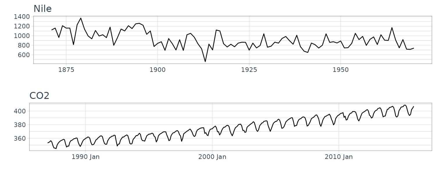
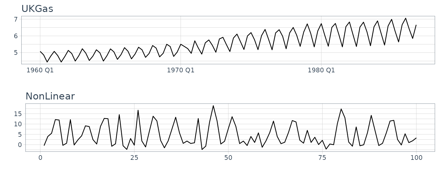
We now convert the data under analysis in the time domain to that in the frequency domain. We will use the following 4 datasets:
And plotting the frequency spectrum:
plot.spectrum <-
  function(dat,
           lab = "",
           sub = "",
           tick = c(8, 4),
           unit = 1
           ) {

    n <- nrow(dat)
    freq_tick <- c(n, tick, 2)

    # Frequency domain transform of data
    dat_FFT <- abs(fft(dat$y)) |>
      as_tibble()

    max_value <- max(dat_FFT$value)

    dat_FFT <- dat_FFT |>
      mutate(
        y = value / max_value,
        f = (0:(n-1)) / n,
        n = 1:n()
      ) |>
      slice(2:(n() / 2 + 1))

    freqs <- dat_FFT$f

    dat_FFT |>
      ggplot(aes(x = f, y = y)) +
      geom_line() +
      ylab("|Standardized frequency spectrum|") +
      xlab(sprintf("Frequency (1/%s)", lab)) +
      ggtitle(paste0(sub, " - num: ", n)) +
      scale_x_continuous(
        labels = sprintf("1/%d", freq_tick),
        breaks = freqs[n / freq_tick * unit]
      ) +
      theme_tq()
  }
# (a) Annual flow of the Nile
plot.spectrum(
Nile,
lab = "Year",
sub = "(a) Nile"
)
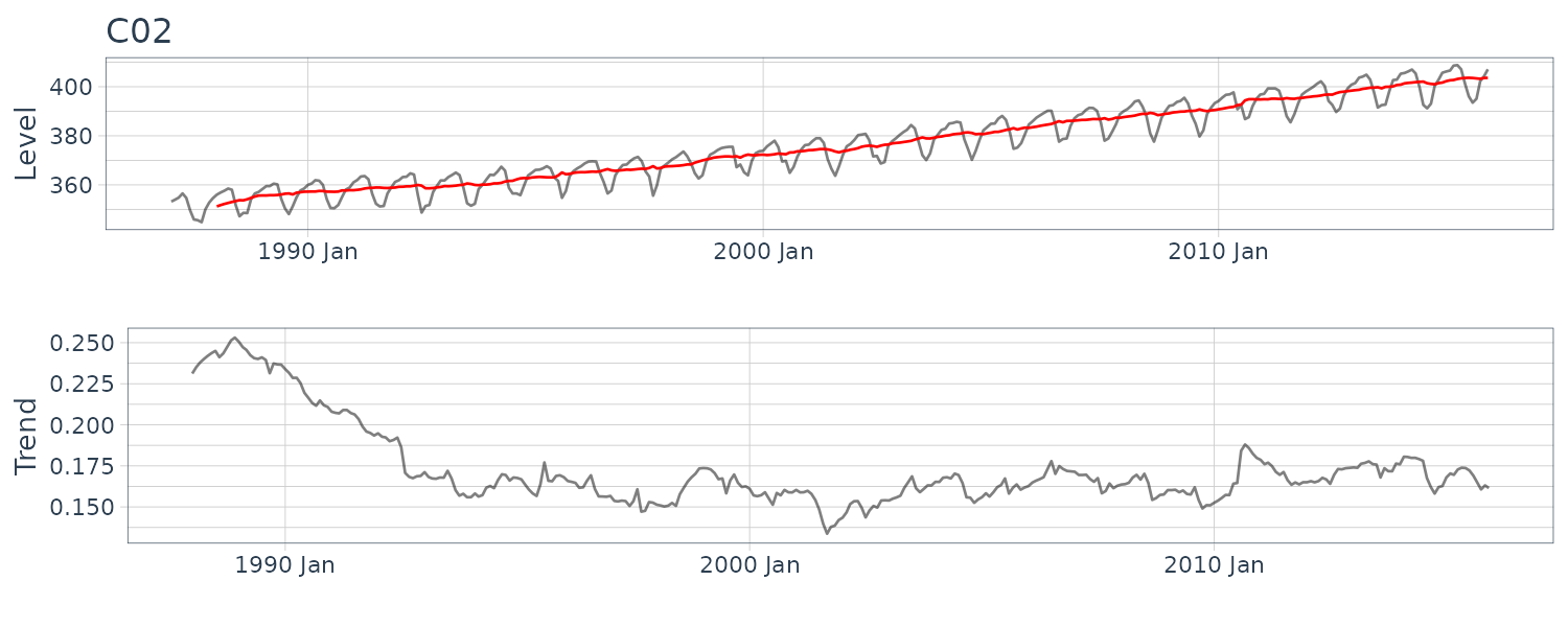
# (b) CO2 concentration in the atmosphere
plot.spectrum(
y_CO2,
lab = "Month",
sub = "(b) CO2",
tick = c(12, 6)
)
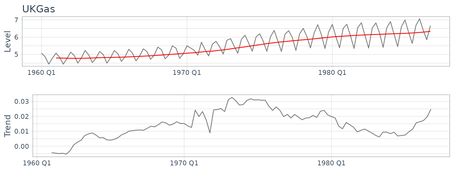
# (c) Quarterly gas consumption in the UK
plot.spectrum(
UKgas,
lab = "Month",
sub = "(c) UKGas",
tick = c(12, 6),
unit = 3
)
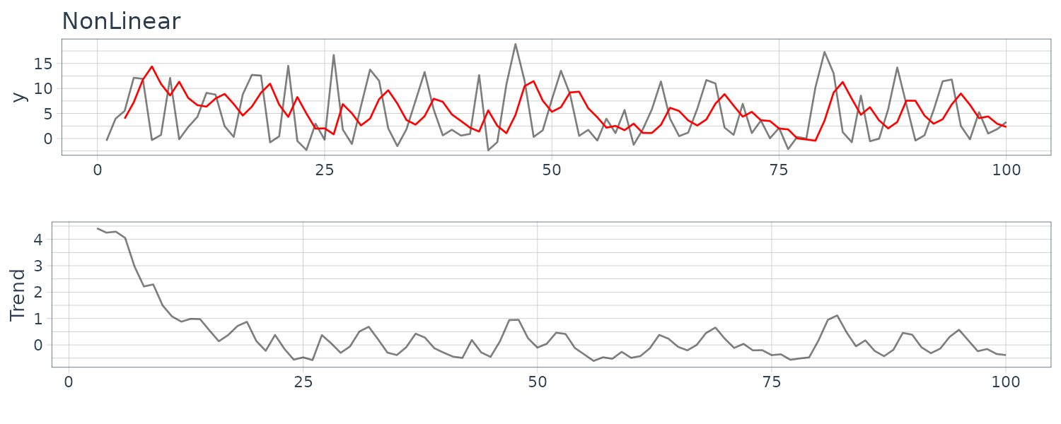
# (d) Artificially-generated data from a nonlinear model
plot.spectrum(
y_nonlinear,
lab = "Time point",
sub = "(d) NonLinear"
)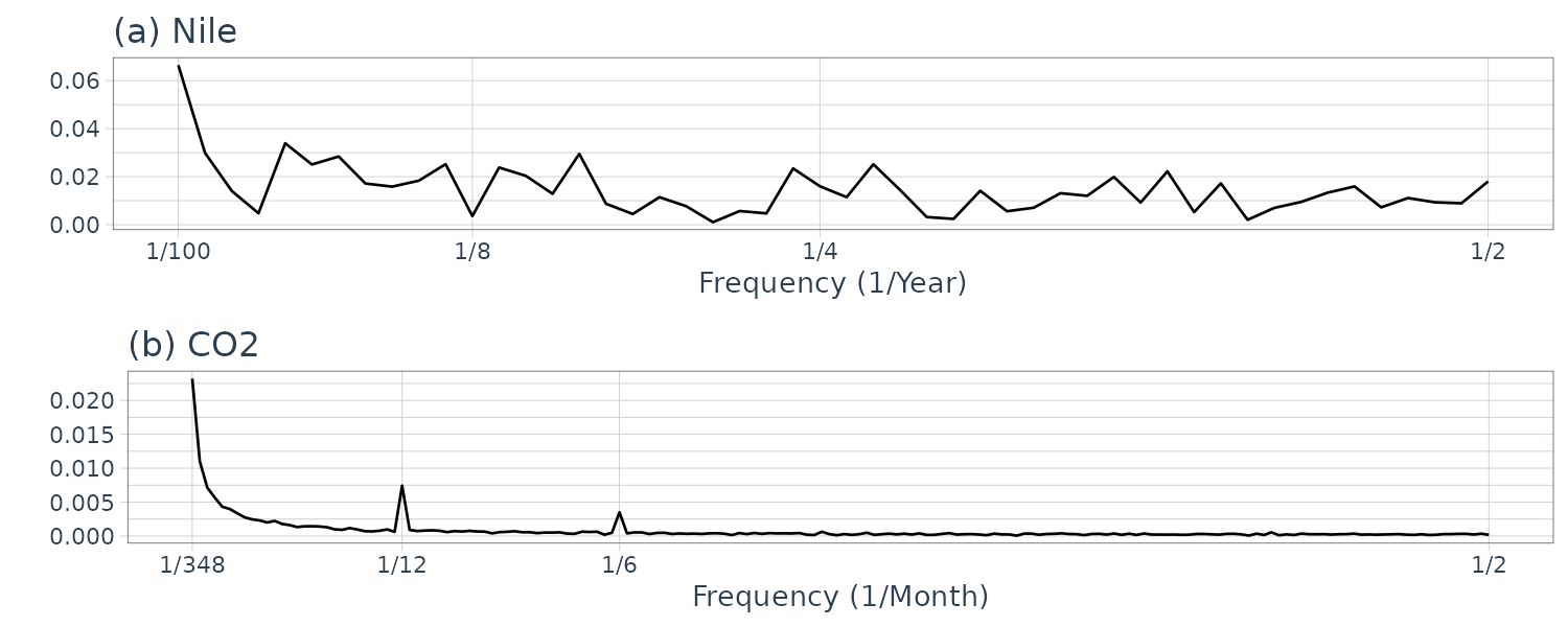
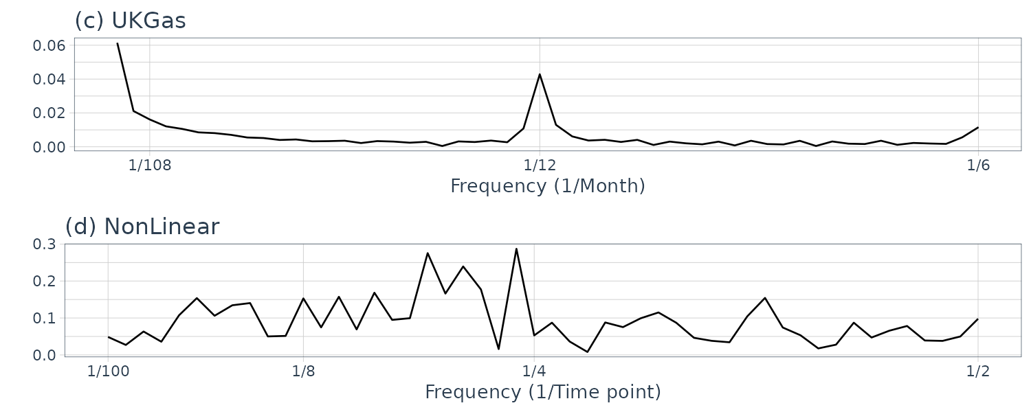
We normalize the absolute value of the frequency spectrum by its maximum value on the vertical axis to understand the contribution of the frequency component easily. Note that we exclude point 0 as it is just the offset but include it in the calculation of max value.
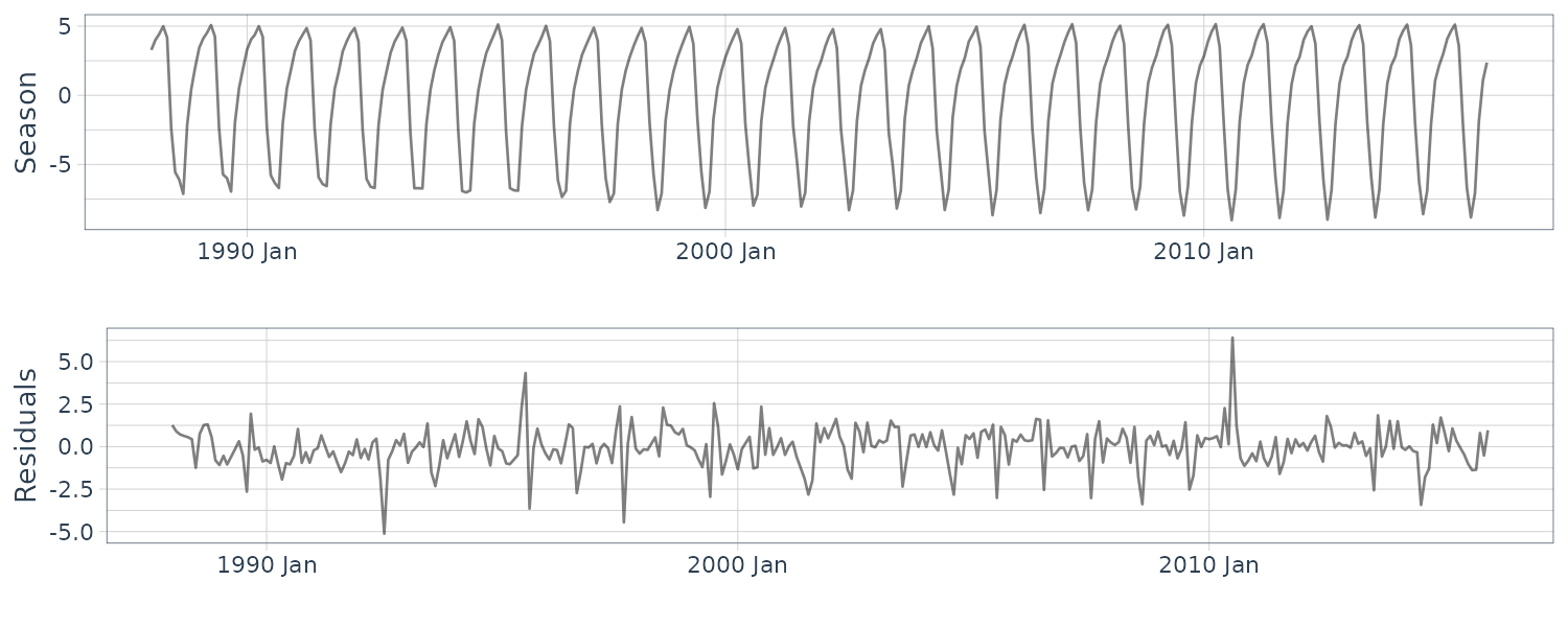
The data (a) appear to contain large values everywhere; hence, we cannot recognize a specific periodicity. The data (b) appear to contain large values at twelve and six months. Since the six-month cycle is incidentally derived from the twelve-month cycle comprising convex and concave halves, we can consider that only the twelve-month period is genuine. The data (c) also have large values at twelve and six months, but we consider that only the twelve-month period is genuine for the same reason. Since the data (d) appear to contain large values everywhere, we cannot recognize a specific periodicity.
Model Definition
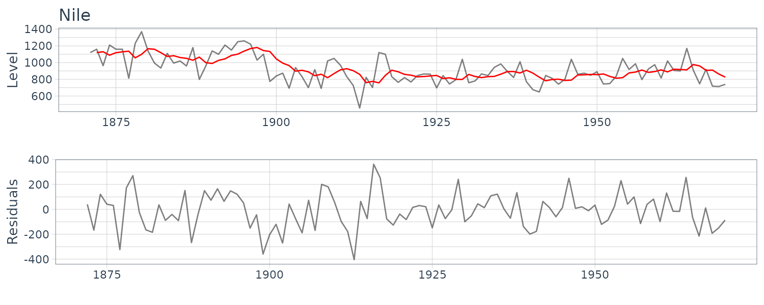
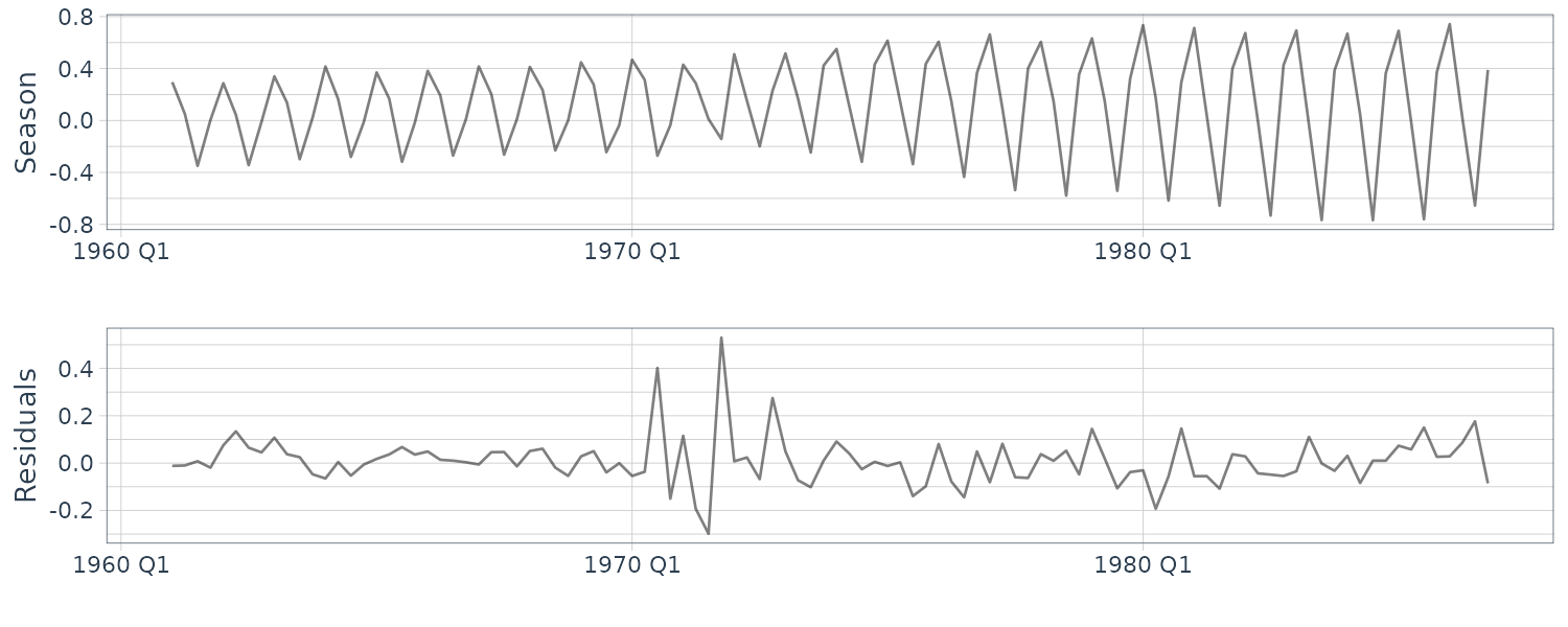
The model is a simple structure expressing the data characteristics. It is common to think of combining simpler structures in defining a model; this is also known as decomposition of time series data. This section explicitly considers “level + trend + season” as a starting point since this is widely recognized as a fundamental decomposition of time series data. Additionally, the remainders resulting from subtracting these estimated components from the original time series data are referred to as residuals.
Holt–Winters method
The Holt–Winters method is a kind of exponentially weighted moving average (EWMA). When observations with a period p are obtained until \(y_{t}\), the k-steps-ahead prediction value \(\hat{y}_{t+k}\) obtained by the additive Holt–Winters method is as follows:
\[\begin{aligned} \hat{y}_{t+k} &= \text{level}_{t} + k\times\text{trend}_{t} + \text{season}_{t-p + k_{p}^{+}}\\ \text{level}_{t} &= \alpha(y_{t} - \text{season}_{t-p}) + (1 - \alpha)(\text{level}_{t-1}+ \text{trend}_{t-1})\\ \text{trend}_{t} &= \beta(\text{level}_{t} - \text{level}_{t-1}) + (1 - \beta)\text{trend}_{t-1}\\ \text{season}_{t} &= \gamma(y_{t} - \text{level}_{t}) + (1 - \gamma)\text{season}_{t-p} \end{aligned}\] \[\begin{aligned} k_{p}^{+} &= \left \lfloor{(k - 1)\text{ mod } p} + 1 \right \rfloor \end{aligned}\]The prediction value \(\hat{y}_{t}\) for k = 0 corresponds to the filtering value. The terms \(\text{level}_{t}, \text{trend}_{t}, \text{season}_{t}\) indicate level component, trend component, and seasonal component, respectively.
The terms \(\alpha, \beta, \gamma\) are an exponential weight for the level, trend, and seasonal component, respectively; they take values from 0 to 1.
While the Holt–Winters method is deterministic, it is known that the method becomes (almost) equivalent to the stochastic method in a specific setting: the equivalence with the autoregressive integrated moving average (ARIMA) model, whereas the equivalence with the state-space model is described later.
In the Holt–Winters method, the exponential weights \(\alpha, \beta, \gamma\) are basic parameters, respectively, and are typically determined to minimize the sum of the squared one-step-ahead prediction error over all time points.
Note that the terms \(\text{level}_{t}, \text{trend}_{t}, \text{season}_{t}\) are just estimates based on the specified parameters. The function HoltWinters() in R is available for the Holt–Winters method; it can perform the specification of parameter values and estimation simultaneously.
Once the model and parameters are specified, we perform the analysis process, i.e., filtering, prediction, and smoothing. This section describes the case of the deterministic Holt–Winters method; we will explain the example of the stochastic state-space model later.
The Holt–Winters method can perform filtering and prediction.
The code for filtering with the Holt–Winters method is as follows:
(a) Annual Flow of the Nile
HW_Nile <- HoltWinters(
  Nile |>
    select(y) |>
    as.ts(),
  beta = FALSE,
  gamma = FALSE
)

> HW_Nile
Holt-Winters exponential smoothing without trend and
without seasonal component.

Call:
HoltWinters(x = as.ts(select(Nile, y)),
  beta = FALSE, gamma = FALSE)

Smoothing parameters:
 alpha: 0.2465579
 beta : FALSE
 gamma: FALSE

Coefficients:
      [,1]
a 805.0389

Nile <- Nile |>
  mutate(
    pred = c(
      NA,
      HW_Nile$fitted[, "xhat"]
    )
  )
(b) CO2 Concentration in the Atmosphere
HW_CO2 <- HoltWinters(
  as.ts(
    y_CO2 |>
      select(y)
  )
)

> HW_CO2
Holt-Winters exponential smoothing with trend and
additive seasonal component.

Call:
HoltWinters(x = as.ts(select(y_CO2, y)))

Smoothing parameters:
 alpha: 0.2447601
 beta : 0.01251553
 gamma: 0.1748568

Coefficients:
           [,1]
a   404.0057970
b     0.1644596
s1    3.0893728
s2    4.0364050
s3    4.7730024
s4    5.1650952
s5    3.5645743
s6   -2.1365395
s7   -6.8188844
s8   -9.0204930
s9   -7.2691087
s10  -1.7723944
s11   1.0173080
s12   2.4942167

y_CO2 <- y_CO2 |>
  mutate(
    pred = c(rep(NA, 12), HW_CO2$fitted[, "xhat"])
  )
Suppose \(N\) is the length of the time series and \(p = 12\). The cofficients represent:
\[\begin{aligned} \begin{bmatrix} a[N]\\ b[N]\\ s[N - 12 + 1]\\ s[N- 12 + 2]\\ \vdots\\ s[N] \end{bmatrix} \end{aligned}\](c) Quarterly Gas Consumption in the UK
HW_UKgas <- HoltWinters(
  UKgas |>
    select(y) |>
    as.ts()
)

> HW_UKgas
Holt-Winters exponential smoothing with trend and
additive seasonal component.

Call:
HoltWinters(x = as.ts(select(UKgas, y)))

Smoothing parameters:
 alpha: 0.02902249
 beta : 1
 gamma: 0.7246027

Coefficients:
          [,1]
a   6.35670491
b   0.02234170
s1  0.76212717
s2  0.08604617
s3 -0.53107110
s4  0.32905534

UKgas <- UKgas |>
  mutate(
    pred = c(
      rep(NA, 4),
      HW_UKgas$fitted[, "xhat"]
    )
  )
(d) Artificial Generated Data from a Nonlinear Model
HW_nonlinear <- HoltWinters(
  y_nonlinear |>
    select(y) |>
    as.ts(),
  gamma = FALSE
)

> HW_nonlinear
Holt-Winters exponential smoothing with trend and
without seasonal component.

Call:
HoltWinters(x = as.ts(select(y_nonlinear, y)),
  gamma = FALSE)

Smoothing parameters:
 alpha: 0.4013391
 beta : 0.1434025
 gamma: FALSE

Coefficients:
       [,1]
a  2.470568
b -0.305886

y_nonlinear <- y_nonlinear |>
  mutate(
    pred = c(
      rep(NA, 2),
      HW_nonlinear$fitted[, "xhat"]
    )
  )
Prediction in R:
nAhead <- 12
dat <- new_data(y_CO2, n = nAhead)

dat$pred <- predict(
  HW_CO2,
  n.ahead = nAhead
)

y_CO2 |>
  autoplot(y) +
  xlab("") +
  geom_line(
    aes(y = pred),
    data = dat,
    col = "blue"
  ) +
  theme_tq()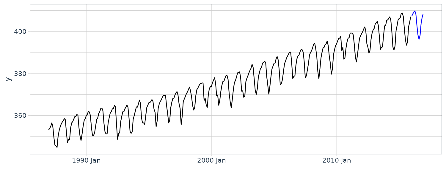
State Space Model
The state-space model interprets series data that have a relation with each other in stochastic terms. First, this model introduces latent random variables that are not directly observed in addition to directly observed data. Such a latent random variable is called a state.
We assume the following association for a state, a Markov property: A state is related only to the state at the previous time point. And an observation at a certain time point depends only on the state at the same time point.
Representation by Graphical Model
The Markov property for the state is expressed by the fact that \(x_{t}\) is directly connected with only its neighbors. In addition, the fact that \(y_{t}\) is directly connected with only \(x_{t}\) indicates an assumption for the observations.
Representation by Probability Distribution
\[\begin{aligned} p(\textbf{x}_{t}|\textbf{x}_{0:t-1}, y_{1:t-1}) &= p(\textbf{x}_{t} | \textbf{x}_{t-1})\\[5pt] p(y_{t}|\textbf{x}_{0:t}, y_{1:t-1}) &= p(y_{t}|\textbf{x}_{t}) \end{aligned}\]The first equation shows that when \(\textbf{x}_{t-1}\) is given, \(\textbf{x}_{t}\) is independent of \(\textbf{x}_{0:t−2}, y_{1:t−1}\). This relation is referred to as conditional independence on state.
The second equation shows that when \(\textbf{x}_{t}\) is given, \(y_{t}\) is independent of \(y_{1:t−1}, \textbf{x}_{0:t−1}\). This relationship is called conditional independence on observations.
Representation by Equation
\[\begin{aligned} \textbf{x}_{t} &= f(\textbf{x}_{t-1}, \textbf{w}_{t}) \end{aligned}\] \[\begin{aligned} y_{t} &= h(\textbf{x}, v_{t}) \end{aligned}\]Where, \(f()\) and \(h()\) are arbitrary functions. \(\textbf{w}_{t}\) and \(v_{t}\) are mutually independent white noise called state noise and observation noise, respectively. The noise \(\textbf{w}_{t}\) is a p-dimensional column vector.
The state equation is a stochastic differential equation for the state. The state noise \(\textbf{w}_{t}\) is the tolerance for a temporal change of state. The state equation potentially specifies a temporal pattern that allows for distortion.
The observation equation, on the contrary, suggests that when observations are obtained from a state, observation noise \(v_{t}\) is added. While the observation noise also has an aspect of supplementing the model definition, it is mostly interpreted as typical noise different from the state noise. The less the observation noise becomes, the more accurate the observations become.
Joint Distribution of State-Space Model
The joint distribution of the state-space model is defined as:
\[\begin{aligned} p(\textbf{x}_{0:T}, y_{1:T}) \end{aligned}\]Transforming the joint distribution:
\[\begin{aligned} p(\textbf{x}_{0:T}, y_{1:T}) &= p(y_{T}, y_{1:T-1}, \textbf{x}_{0:T})\\[5pt] &= p(y_{T}|y_{1:T-1}, \textbf{x}_{0:T})p(y_{1:T-1}, \textbf{x}_{0:T})\\[5pt] &= p(y_{T}|y_{1:T-1}, \textbf{x}_{0:T})p(\textbf{x}_{T}, \textbf{x}_{0:T-1}, y_{1:T-1})\\[5pt] &= p(y_{T}|y_{1:T-1}, \textbf{x}_{0:T})p(\textbf{x}_{T}| \textbf{x}_{0:T-1}, y_{1:T-1})p(\textbf{x}_{0:T-1},y_{1:T-1})\\[5pt] &\ \ \vdots\\ &= \Big[\prod_{t=2}^{T}p(y_{t}|y_{1:t-1}, \textbf{x}_{0:t})p(\textbf{x}_{t}|\textbf{x}_{0:t-1}, y_{1:t-1})\Big]p(\textbf{x}_{0:1}, y_{1})\\ &= \Big[\prod_{t=2}^{T}p(y_{t}|y_{1:t-1}, \textbf{x}_{0:t})p(\textbf{x}_{t}|\textbf{x}_{0:t-1}, y_{1:t-1})\Big]p(y_{1}|\textbf{x}_{0:1})p(\textbf{x}_{1}|\textbf{x}_{0})p(\textbf{x}_{0})\\ &= p(\textbf{x}_{0})\Big[\prod_{t=2}^{T}p(y_{t}|\textbf{x}_{t})p(\textbf{x}_{t}|\textbf{x}_{t-1})\Big]p(y_{1}|\textbf{x}_{1})p(\textbf{x}_{1}|\textbf{x}_{0})\\ &= p(\textbf{x}_{0})\prod_{t=1}^{T}p(y_{t}|\textbf{x}_{t})p(\textbf{x}_{t}|\textbf{x}_{t-1}) \end{aligned}\]The above equation simply states that the state-space model is determined by a simple product by assumed prior distribution \(p(\textbf{x}_{0})\), observation equation \(p(y_{t}\mid \textbf{x}_{t})\), and state equation \(p(\textbf{x}_{t}\mid \textbf{x}_{t−1})\). This result is a natural consequence of the assumptions for the state space model.
Features of State-Space Model
The state, enables the state-space model to be used as the basis for easily constructing a complicated model by combining multiple states. Recall that we can arbitrarily choose a state convenient for interpretation. Such a framework improves the flexibility of modeling.
Next, the state-space model represents the relation among observations via states indirectly rather than by direct connection among observations. This feature contrasts with the ARMA model (autoregressive moving average model) which directly represents the relation among observations. The ARMA(p, q) model is a stochastic one often used in time series analysis and is defined as:
\[\begin{aligned} y_{t} &= \sum_{j=1}^{p}\phi_{j}y_{t-j} + \sum_{j=1}^{q}\theta_{j} e_{t-j} + e_{t} \end{aligned}\]The ARMA model for the d-th differences time series becomes an ARIMA model (autoregressive integrated moving average model) and is denoted by ARIMA( p, d, q).
The ARIMA and state-space models are closely related. The models often used in the state-space model can be defined as the ARIMA model, and the ARIMA model can also be defined as one of the state-space models.
There is no essential difference between the two models from the viewpoint of capturing the temporal pattern of data stochastically. However, their underlying philosophies are different. Since the ARIMA model represents the relation among observations directly, the modeling problem requires a black box approach. On the contrary, since the state-space model represents the relation among observations indirectly in terms of states, the modeling problem results in a white box approach. The analyst assumes as much as possible regarding the factors generating the association among data and reflects them in the model through the corresponding latent variables.
It is also well recognized that the state-space model is equivalent to the hidden Markov model, which has been developed primarily in speech recognition. However, the random variable to be estimated in the hidden Markov model is discrete.
Classification of State-Space Models
If either f or h is a nonlinear function and either \(\textbf{w}_{t}\) or \(v_{t}\) has a non-Gaussian distribution, then the state-space model is referred to as a nonlinear non-Gaussian state-space model.
If either f or h is a nonlinear function and both \(w_{t}\) and \(v_{t}\) have Gaussian distributions, then the state-space model is referred to as a nonlinear Gaussian state-space model.
If both f and h are linear functions and either \(\textbf{w}_{t}\) or \(v_{t}\) has a non-Gaussian distribution, then the state-space model is referred to as a linear non-Gaussian state-space model.
Furthermore, if both f and h are linear functions and both \(\textbf{w}_{t}\) and \(v_{t}\) have Gaussian distributions, then the state-space model is referred to as a linear Gaussian state-space model.
Linear Gaussian State-Space Model
The state equation and observation equation for the linear Gaussian state-space model are expressed as follows:
\[\begin{aligned} \textbf{x}_{t} &= \textbf{G}_{t}\textbf{x}_{t-1} + \textbf{w}_{t} \end{aligned}\] \[\begin{aligned} y_{t} &= \textbf{F}_{t}\textbf{x}_{t} + v_{t} \end{aligned}\] \[\begin{aligned} \textbf{w}_{t} &\sim N(\textbf{0}, \textbf{W}_{t})\\ v_{t} &\sim N(0, V_{t}) \end{aligned}\]Where \(\textbf{G}_{t}\) is a p × p state transition matrix, \(\textbf{F}_{t}\) is a 1 × p observation matrix, \(\textbf{W}_{t}\) is a p × p covariance matrix for the state noise, and \(V_{t}\) is a variance for the observation noise.
The prior distribution is also expressed as:
\[\begin{aligned} \textbf{x}_{0} &\sim N(\textbf{m}_{0}, \textbf{C}_{0}) \end{aligned}\]Where \(\textbf{m}_{0}\) is the p-dimensional mean vector and \(\textbf{C}_{0}\) is a p × p covariance matrix.
In addition, the above equations can be expressed equivalently with a probability distribution as follows:
\[\begin{aligned} p(\textbf{x}_{t} | \textbf{x}_{t-1}) &= N(\textbf{G}_{t}\textbf{x}_{t-1}, \textbf{W}_{t})\\[5pt] p(y_{t}|\textbf{x}_{t}) &= N(\textbf{F}_{t}\textbf{x}_{t}, V_{t})\\[5pt] p(\textbf{x}_{0}) &= N(\textbf{m}_{0}, \textbf{C}_{0}) \end{aligned}\]Parameters in the linear Gaussian state-space model are summarized as:
\[\begin{aligned} \boldsymbol{\theta} &= \{\textbf{G}_{t}, \textbf{F}_{t}, \textbf{W}_{t}, V_{t}, \textbf{m}_{0}, \textbf{C}_{0}\} \end{aligned}\]The linear Gaussian state-space model is also referred to as a dynamic linear model (DLM).
State Estimation in the State-Space Model
The state in the state-space model is estimated based on observations through the current time point t. Thus, the distribution to be estimated becomes a conditional distribution (posterior distribution of the state) as:
\[\begin{aligned} p(\text{state} | y_{1:t}) \end{aligned}\]We must first consider all time points known as the joint posterior distribution of the state:
\[\begin{aligned} p(\textbf{x}_{0}, \textbf{x}_{0}, \cdots, \textbf{x}_{t'}, \cdots | y_{1:t}) \end{aligned}\]The estimation type is classified depending on the focused time point \(t'\):
\[\begin{aligned} \begin{cases} \text{smoothing} & t' < t\\ \text{filtering} & t' = t\\ \text{prediction} & t' > t \end{cases} \end{aligned}\]If we want to exclude the states whose time points differ from the focused \(t'\), we perform marginalization as:
\[\begin{aligned} p(\textbf{x}_{t'} | y_{1:t}) &= \int p(\textbf{x}_{0}, \textbf{x}_{0}, \cdots, \textbf{x}_{t'}, \cdots | y_{1:t})\ d\textbf{x}_{\text{except }t'} \end{aligned}\]Known as the marginal posterior distribution of the state.
A Simple Example
Let there be a domestic cat with a collar with a GPS tracker function for monitoring its behavior. We assume a case wherein the cat moves straight away from home at an average speed \(v\). We formulate this problem in terms of the linear Gaussian state-space model as:
\[\begin{aligned} x_{t} &= x_{t-1} + v + w_{t} \end{aligned}\] \[\begin{aligned} y_{t} &= x_{t}+ v_{t} \end{aligned}\] \[\begin{aligned} w_{t} &\sim N(0, \sigma_{w}^{2})\\ v_{t} &\sim N(0, \sigma^{2}) \end{aligned}\]Where \(p(x_{0}) \sim N(m_{0}, C_{0})\) and \(m_{0} = \hat{m}_{1}\) is the guessed position at \(t = 1\) based on prior knowledge, and variance \(C_{0}\) represents the degree of confidence in the guess. \(x_{t}\) is the cat’s position at time point t, \(v\) is the average velocity (constant), \(w_{t}\) is the fluctuation in velocity during movement, \(y_{t}\) is an observation at time t, and \(v_{t}\) is the noise at the observation.
We derive the process of obtaining the state sequentially. We first estimate the cat’s position at the beginning of movement, i.e., at t = 1 when observation starts. Based on prior knowledge, we multiply the prior distribution, \(p(x_{1})\), by the likelihood, \(p(y_{1}\mid x_{1})\), based on observation to obtain the posterior distribution, \(p(x_{1}\mid y_{1})\) (Bayesian updating).
Since the consideration of likelihood increases the accuracy, the variance of the posterior distribution is smaller than that of the prior distribution. This posterior distribution is the result of estimating where the cat is at the beginning of the observation.
Subsequently, we estimate the cat’s position at the next time point t = 2 after it moves. The prior distribution, \(p(x_{2})\) corresponds to the posterior distribution at t = 1, \(p(x_{1}\mid y_{1})\). Since the cat is moving at this time, we reflect the movement in this prior distribution (state transition) based on the average speed. The variance of the one-step-ahead predictive distribution is unavoidably greater than that of the prior distribution because a fluctuation \(w_{t}\) in the moving speed increases the uncertainty of the movement. This one-step-ahead predictive distribution predicts the situation after the movement. Hence, we multiply this predictive distribution by the likelihood based on the observation at t = 2, \(p(y_{2}\mid x_{2})\), resulting in a posterior distribution (Bayesian updating). Since the consideration of likelihood increases the accuracy, the variance of the posterior distribution is less than that of the one-step-ahead predictive distribution, \(p(x_{2}\mid y_{1})\). This posterior distribution, \(p(x_{2}\mid y_{2})\) is the result of estimating where the cat is at the next time point.
First, Bayesian updating at time point t = 1 is expressed as:
\[\begin{aligned} p(x_{1} | y_{1}) &\propto p(x_{1}) \times p(y_{1} | x_{1})\\ &= \frac{1}{\sqrt{2\pi C_{0}}}e^{-\frac{(x_{1} - m_{0})^{2}}{2C_{0}}}\times \frac{1}{\sqrt{2\pi \sigma^{2}}}e^{-\frac{(y_{1} - x_{1})^{2}}{2\sigma^{2}}}\\ & \propto e^{-\frac{x_{1}^{2} - 2m_{0}x_{1}}{2C_{0}} - \frac{-2y_{1}x_{1} + x_{1}^{2}}{2\sigma^{2}}}\\ &= e^{-\Big(\frac{1}{2C_{0}} + \frac{1}{2\sigma^{2}}\Big)x_{1}^{2} + \Big(\frac{2m_{0}x_{1}}{2C_{0}} + \frac{2y_{1}x_{1}}{2\sigma^{2}}\Big)}\\ &= e^{-\frac{1}{2}\Big(\frac{1}{C_{0}} + \frac{1}{\sigma^{2}}\Big)x_{1}^{2} + \Big(\frac{m_{0}}{C_{0}} + \frac{y_{1}}{\sigma^{2}}\Big)x_{1}} \end{aligned}\]The posterior distribution at \(t = 1\) can also be expressed as follows:
\[\begin{aligned} p(x_{1}|y_{1}) &= \frac{1}{\sqrt{2\pi C_{1}}}e^{-\frac{(x_{1} - m_{1})^{2}}{2C_{1}}}\\ &\propto e^{-\frac{x_{1}^{2} - 2m_{1}x_{1}}{2C_{1}}}\\ &= e^{-\frac{1}{2}\frac{1}{C_{1}}x_{1}^{2} + \frac{m_{1}}{C_{1}}x_{1}} \end{aligned}\]Equating the two yields the following relationships:
\[\begin{aligned} \frac{1}{C_{1}} &= \frac{1}{C_{0}} + \frac{1}{\sigma^{2}} \end{aligned}\]And:
\[\begin{aligned} m_{1} &= C_{1}\frac{1}{C_{0}}m_{0} + C_{1}\frac{1}{\sigma^{2}}y_{1}\\[10pt] &= \frac{\frac{1}{C_{0}}}{\frac{1}{C_{0}} + \frac{1}{\sigma^{2}}}m_{0} + \frac{\frac{1}{\sigma^{2}}}{\frac{1}{C_{0}} + \frac{1}{\sigma^{2}}}y_{1}\\[10pt] &= \frac{\sigma^{2}m_{0} + C_{0}y_{1}}{\sigma^{2} + C_{0}}\\[10pt] &= \frac{\sigma^{2} + C_{0} - C_{0}}{\sigma^{2} + C_{0}}m_{0} + \frac{C_{0}}{\sigma^{2} + C_{0}}y_{1}\\[10pt] &= m_{0} + \frac{C_{0}}{\sigma^{2} + C_{0}}(y_{1} - m_{0}) \end{aligned}\]The first equation shows that the precision (the inverse of the variance of the posterior distribution) is the sum of the precisions of the prior distribution and the precison of the likelihood. Such a fact implies that the precision or variance always increases or decreases through Bayesian updating because the certainty increases by considering observations. On the contrary, the second equation shows that the mean for the posterior distribution is a weighted sum of the means for prior distribution and the likelihood; each weight is proportional to each precision:
\[\begin{aligned} \frac{\sigma^{2} + C_{0} - C_{0}}{\sigma^{2} + C_{0}}m_{0} + \frac{C_{0}}{\sigma^{2} + C_{0}}y_{1} \end{aligned}\]From the state equation:
\[\begin{aligned} x_{t} &= x_{t-1} + v + w_{t}\\ \hat{C}_{2} &= \text{var}(x_{1}) + \text{var}(v) + \text{var}(w_{2})\\ &= C_{1} + 0 + \sigma_{w}^{2}\\ &= C_{1}+ \sigma_{w}^{2}\\[5pt] \hat{m}_{2} &= E[x_{1}] + E[v] + E[w_{2}]\\ &= m_{1} + v + 0\\ &= m_{1} + v \end{aligned}\]The above expression shows that the variance always increases with the state transition.
Recall that:
\[\begin{aligned} m_{0} &= \hat{m}_{1} \end{aligned}\]We confirm the Bayesian updating at time point t = 2. Since the mechanism of Bayesian updating remains the same as that at t = 1, we can obtain the result by replacing:
\[\begin{aligned} m_{1} &= \hat{m}_{2}\\ C_{1} &= \hat{C}_{2} \end{aligned}\]Specifically, the Bayesian updating at time point t = 2 is as follows:
\[\begin{aligned} \frac{1}{C_{2}} &= \frac{1}{C_{1}} + \frac{1}{\sigma^{2}}\\ &= \frac{1}{\hat{C}_{2}} + \frac{1}{\sigma^{2}}\\ &= \frac{1}{C_{1} + \sigma_{w}^{2}} + \frac{1}{\sigma^{2}}\\ \end{aligned}\] \[\begin{aligned} m_{2} &= m_{1} + \frac{C_{1}}{\sigma^{2} + C_{1}}(y_{2} - m_{1})\\ &= \hat{m}_{2} + \frac{\hat{C_{2}}}{\sigma^{2} + \hat{C}_{2}}(y_{2} - \hat{m_{2}})\\ &= (m_{1} + v) + \frac{C_{1} + \sigma_{w}^{2}}{\sigma^{2} + C_{1} + \sigma_{w}^{2}}[y_{2} - (m_{1} + v)] \end{aligned}\]The above result corresponds to a simple example of Kalman filtering. We subsequently supplement \(m_{2}\) for estimating the mean. This equation has a prediction-error correction structure: the mean \(\hat{m}_{2}\) for the one-step-ahead predictive distribution, \(p(x_{2}\mid y_{1})\) is corrected by observations \(y_{2}\). This structure is a general result obtained by the combination of state transition and Bayesian updating. In addition, the equation can take the form:
\[\begin{aligned} x_{1}y_{t} + (1 − x_{1})\hat{m}_{2} \end{aligned}\]Therefore, it also has a structure of an exponentially weighted moving average.
Formulation of Filtering Distribution
We now formulate the recursions for the marginal posterior distribution of the state.
For filtering, \(t'= t\) is set:
\[\begin{aligned} p(\textbf{x}_{t} | y_{1:t}) &= \int p(\textbf{x}_{0}, \textbf{x}_{0}, \cdots, \textbf{x}_{t}, \cdots | y_{1:t})\ d\textbf{x}_{\text{except }t} \end{aligned}\]Note the relation:
\[\begin{aligned} p(a, b | c) &= p(a | b, c)p(b |c) \end{aligned}\]We can show the derivation of the above relation. Using the product rule of probability to \(p(a, b, c)\) considering \(a, b\) as a single block:
\[\begin{aligned} p(a, b | c) &= p(a, b | c)p(c) \end{aligned}\]Now, using the product rule of probability to \(p(a, b, c)\) considering \(b, c\) as a single block:
\[\begin{aligned} p(a, b, c) &= p(a | b, c)p(b, c) \end{aligned}\]Apply the product rule to the last term \(p(b, c)\):
\[\begin{aligned} p(a, b, c) &= p(a | b, c)p(b | c)p(c) \end{aligned}\]Thus:
\[\begin{aligned} p(a, b, c) &= p(a | b, c)p(b | c)p(c)\\[10pt] p(a, b | c)p(c) &= p(a | b, c)p(b | c)p(c)\\[10pt] p(a, b | c) &= p(a | b, c)p(b | c) \end{aligned}\]The filtering distribution becomes:
\[\begin{aligned} p(\mathbf{x}_{t} | y_{1:t}) &= p(\mathbf{x}_{t} | y_{t}, y_{1:t-1})\\[10pt] &= \frac{p(\mathbf{x}_{t}, y_{t}|y_{1:t-1})}{p(y_{t}|y_{1:t-1})}\\[10pt] &= \frac{p(y_{t}, \mathbf{x}_{t}|y_{1:t-1})}{p(y_{t}|y_{1:t-1})} \end{aligned}\]Using the relation above:
\[\begin{aligned} \frac{p(y_{t}, \mathbf{x}_{t}|y_{1:t-1})}{p(y_{t}|y_{1:t-1})} &= \frac{p(y_{t}| \mathbf{x}_{t}, y_{1:t-1})p(\mathbf{x}_{t}|y_{1:t-1})}{p(y_{t}|y_{1:t-1})} \end{aligned}\]From the conditional independence:
\[\begin{aligned} \frac{p(y_{t}| \mathbf{x}_{t}, y_{1:t-1})p(\mathbf{x}_{t}|y_{1:t-1})}{p(y_{t}|y_{1:t-1})} &= \frac{p(y_{t}| \mathbf{x}_{t})p(\mathbf{x}_{t}|y_{1:t-1})}{p(y_{t}|y_{1:t-1})}\\ \end{aligned}\]Hence:
\[\begin{aligned} p(\mathbf{x}_{t} | y_{1:t}) &= \frac{p(y_{t}| \mathbf{x}_{t})p(\mathbf{x}_{t}|y_{1:t-1})}{p(y_{t}|y_{1:t-1})}\\ \end{aligned}\]Where \(p(\mathbf{x}_{t}\mid y_{1:t-1})\) is referred to as the one-step-ahead predictive distribution.
And \(p(y_{t}\mid y_{1:t-1})\) is known as the one-step-ahead predictive likelihood.
Expanding the one-step predictive distribution:
\[\begin{aligned} p(\textbf{x}_{t}|y_{1:t-1}) &= \int p(\textbf{x}_{t}, \textbf{x}_{t-1} | y_{1:t-1})\ d\textbf{x}_{t-1}\\ &= \int p(\textbf{x}_{t} | \textbf{x}_{t-1}, y_{1:t-1})p(\textbf{x}_{t-1}|y_{1:t-1})\ d\textbf{x}_{t-1}\\ &= \int p(\textbf{x}_{t} | \textbf{x}_{t-1})p(\textbf{x}_{t-1}|y_{1:t-1})\ d\textbf{x}_{t-1} \end{aligned}\]Expanding the one-step predictive likelihood:
\[\begin{aligned} p(y_{t}|y_{1:t-1}) &= \int p(y_{t}, \textbf{x}_{t} | y_{1:t-1})\ d\textbf{x}_{t}\\ &= \int p(y_{t}|\textbf{x}_{t}, y_{1:t-1})p(\textbf{x}_{t}|y_{1:t-1})\ d\textbf{x}_{t}\\ &= \int p(y_{t}|\textbf{x}_{t})p(\textbf{x}_{t}|y_{1:t-1})\ d\textbf{x}_{t} \end{aligned}\]The filtering distribution:
\[\begin{aligned} p(\textbf{x}_{t} | y_{1:t}) &= p(\textbf{x}_{t}|y_{1:t-1})\frac{p(y_{t}|\textbf{x}_{t})}{p(y_{t}|y_{1:t-1})} \end{aligned}\]The one-step-ahead predictive distribution is corrected based on the likelihood.
One-step-ahead predictive distribution:
\[\begin{aligned} p(\textbf{x}_{t} | y_{1:t-1}) &= \int p(\textbf{x}_{t}|\textbf{x}_{t-1})p(\textbf{x}_{t-1}|y_{1:t-1})\ d\textbf{x}_{t-1} \end{aligned}\]The filtering distribution one time before is transitioned in the time-forward direction based on the state equation.
One-step-ahead predictive likelihood:
\[\begin{aligned} p(y_{t}|y_{1:t-1}) &= \int p(y_{t}|\textbf{x}_{t})p(\textbf{x}_{t}|y_{1:t-1})\ d\textbf{x}_{t} \end{aligned}\]The one-step-ahead predictive distribution is converted in the domain of observations based on the observation equation; this likelihood also corresponds to the normalization factor for the numerators in the filtering distribution.
Filtering can be achieved by:
- obtaining the one-step-ahead predictive distribution through the state transition from the filtering distribution one time before
- correcting the obtained distribution based on the observations
Formulation of Predictive Distribution
We now consider k-steps-ahead prediction with \(t' = t + k\) in:
\[\begin{aligned} p(\textbf{x}_{t + k} | y_{1:t}) &= \int p(\textbf{x}_{0}, \textbf{x}_{0}, \cdots, \textbf{x}_{t+k}, \cdots | y_{1:t})\ d\textbf{x}_{\text{except }t + k} \end{aligned}\]The corresponding k-steps-ahead predictive distribution is:
\[\begin{aligned} p(\textbf{x}_{t+k} | y_{1:t}) &= \int p(\textbf{x}_{t+k}, \textbf{x}_{t+k-1}|y_{1:t})\ d\textbf{x}_{t+k-1}\\ &= \int p(\textbf{x}_{t+k} | \textbf{x}_{t+k-1}, y_{1:t})p(\textbf{x}_{t+k-1}|y_{1:t})\ d\textbf{x}_{t+k-1}\\ &= \int p(\textbf{x}_{t+k}|\textbf{x}_{t+k-1})p(\textbf{x}_{t+k-1}|y_{1:t})\ d\textbf{x}_{t+k-1} \end{aligned}\]The (k−1)-steps-ahead predictive distribution is transitioned in the forward time direction based on the state equation. The (k−2)-steps-ahead predictive distribution is transitioned in the forward time direction based on the state equation. And etc.
Starting from the one-step-ahead predictive distribution and repeating the transition in the forward time direction k − 1 times based on the state equation, we obtain the k-steps-ahead predictive distribution.
Recall that if the filtering distribution one time before is transitioned in the forward time direction based on the state equation, we can obtain the one-step-ahead predictive distribution, \(p(x_{t}\mid y_{1:t-1})\). Therefore, we can conclude as follows: Starting from the filtering distribution \(p(x_{t} \mid y_{1:t})\) and repeating the transition in the forward time direction k times based on the state equation, we obtain the k-steps-ahead predictive distribution.
Comparing the k-steps-ahead prediction with filtering, we can see that the state transition (horizontal arrow) is repeated without correction based on the observations (vertical arrow). Hence, while the accuracy of prediction gradually decreases as k increases, the most likely distributions continue to be generated based on the information through the filtering point. Incidentally, the state-space model applies this concept directly to the missing observations. Therefore, the missing observations in the state-space model are compensated for with prediction values. This is the background showing that it is easy to handle missing observations in the state-space model.
Formulation of the Smoothing Distribution
We now consider smoothing. This book focuses on the popular fixed-interval smoothing; Hence, we replace the \(t, t'\) with T and t, respectively in \(p(\textbf{x}_{t'} \mid y_{1:t})\). In this case, the smoothing distribution is \(p(\textbf{x}_{t} \mid y_{1:T})\).
To perform smoothing, we first assume that filtering has been completed through the time point T . In addition, we assume that sequential updating in the reverse time direction. The recursive formulas for the smoothing distribution require expressing the element about t + 1 clearly. Hence, we deform the smoothing distribution to ensure that the element \(x_{t+1}\) can be expressed explicitly as follows:
\[\begin{aligned} p(\textbf{x}_{t} | y_{1:T}) &= \int p(\textbf{x}_{t}, \textbf{x}_{t+1}|y_{1:T})\ d\textbf{x}_{t+1}\\ &= \int p(\textbf{x}_{t}| \textbf{x}_{t+1}, y_{1:T})p(\textbf{x}_{t+1}|y_{1:T})\ d\textbf{x}_{t+1}\\ &= \int p(\textbf{x}_{t+1}|y_{1:T})p(\textbf{x}_{t}| \textbf{x}_{t+1}, y_{1:T})\ d\textbf{x}_{t+1}\\ &= \int p(\textbf{x}_{t+1}|y_{1:T})p(\textbf{x}_{t}| \textbf{x}_{t+1}, y_{1:t})\ d\textbf{x}_{t+1}\\ &= \int p(\textbf{x}_{t+1}|y_{1:T})\frac{p(\textbf{x}_{t}, \textbf{x}_{t+1}|y_{1:t})}{p(\textbf{x}_{t+1}|y_{1:t})}\ d\textbf{x}_{t+1}\\[10pt] &= \int p(\textbf{x}_{t+1}|y_{1:T})\frac{p(\textbf{x}_{t+1}, \textbf{x}_{t}|y_{1:t})}{p(\textbf{x}_{t+1}|y_{1:t})}\ d\textbf{x}_{t+1}\\[10pt] &= \int p(\textbf{x}_{t+1}|y_{1:T})\frac{p(\textbf{x}_{t+1}| \textbf{x}_{t},y_{1:t})p(\textbf{x}_{t}|y_{1:t})}{p(\textbf{x}_{t+1}|y_{1:t})}\ d\textbf{x}_{t+1} \end{aligned}\]\(p(\textbf{x}_{t} \mid y_{1:t})\) in the numerator does not depend on \(\textbf{x}_{t+1}\):
\[\begin{aligned} \int p(\textbf{x}_{t+1}|y_{1:T})\frac{p(\textbf{x}_{t+1}| \textbf{x}_{t},y_{1:t})p(\textbf{x}_{t}|y_{1:t})}{p(\textbf{x}_{t+1}|y_{1:t})}\ d\textbf{x}_{t+1} &= p(\textbf{x}_{t}|y_{1:t})\int p(\textbf{x}_{t+1}|y_{1:T})\frac{p(\textbf{x}_{t+1}| \textbf{x}_{t},y_{1:t})}{p(\textbf{x}_{t+1}|y_{1:t})}\ d\textbf{x}_{t+1}\\[10pt] &= p(\textbf{x}_{t}|y_{1:t})\int p(\textbf{x}_{t+1}|y_{1:T})\frac{p(\textbf{x}_{t+1}| \textbf{x}_{t})}{p(\textbf{x}_{t+1}|y_{1:t})}\ d\textbf{x}_{t+1} \end{aligned}\]The filtering distribution is corrected based on the smoothing distribution at one time ahead. Hence, the following relation continues to hold in a chain:
- Smoothing distribution at time point T − 1: the filtering distribution at time point T − 1 is corrected based on the smoothing distribution at time point T
- Smoothing distribution at time point T − 2: the filtering distribution at time point T − 2 is corrected based on the smoothing distribution at time point T − 1
- …
Likelihood and Model Selection in the State-Space Model
The likelihood for an entire time series can be decomposed as follows:
\[\begin{aligned} p(y_{1}, y_{2}, \cdots, y_{T};\boldsymbol{\theta}) &= p(y_{1:T};\boldsymbol{\theta})\\ &= p(y_{T}, y_{1:T-1};\boldsymbol{\theta})\\ &= p(y_{T}|y_{1:T-1};\boldsymbol{\theta})p(y_{1:T-1};\boldsymbol{\theta})\\ &\ \ \vdots\\ &= \prod_{t=1}^{T}p(y_{t}|y_{1:t-1};\boldsymbol{\theta}) \end{aligned}\]Where \(y_{1:0}\) does not exist and is assumed to be the empty set \(\emptyset\):
\[\begin{aligned} p(y_{1}|y_{1:0}; \boldsymbol{\theta}) &= p(y_{1}|\emptyset; \boldsymbol{\theta})\\ &= p(y_{1};\boldsymbol{\theta}) \end{aligned}\]Taking the logarithm of the likelihood yields the log-likelihood as:
\[\begin{aligned} l(\boldsymbol{\theta}) &= \log p(y_{1:T};\boldsymbol{\theta})\\ &= \sum_{t=1}^{T}\log p(y_{t}|y_{1:t-1};\boldsymbol{\theta}) \end{aligned}\]We see that the log-likelihood for the entire time series can be represented as the sum of the logarithms of the one-step-ahead predictive likelihoods. Recalling that the filtering recursion derives the one-step-ahead predictive likelihood during its processing, we see that the likelihood can be calculated efficiently through filtering.
When Parameters are Not Regarded as Random Variables
The approach is based on frequentism. In this case, before estimating the time series, we typically specify the point estimates for the parameter using the maximum likelihood method.
A maximum likelihood estimator \(\hat{\boldsymbol{\theta}}\) for the parameters in the state-space model is expressed as follows:
\[\begin{aligned} \hat{\boldsymbol{\theta}} &= \underset{\boldsymbol{\theta}}{\text{argmax }} l(\boldsymbol{\theta})\\ &= \underset{\boldsymbol{\theta}}{\text{argmax }} \log p(y_{1:T};\boldsymbol{\theta})\\ &= \underset{\boldsymbol{\theta}}{\text{argmax }} \sum_{t=1}^{T}\log p(y_{t}|y_{1:t-1};\boldsymbol{\theta}) \end{aligned}\]We obtain the maximum likelihood estimator for parameters based on a particular number of observations. This is achieved through several methods: a direct search for different values of parameters, quasi-Newton method, when a numerical optimization is applicable, and the expectation maximization (EM) algorithm.
When Parameters are Regarded as Random Variables
The approach is based on Bayesianism. Unlike the case of frequentism, treating parameters as random variables makes it possible to consider their uncertainties more appropriately. In this case, for the estimation of a time series, Bayesian estimation is applied to both parameters and state.
We treat the augmented \(\text{state} = \{\textbf{x}, \boldsymbol{\theta}\}\) comprising the original state \(\textbf{x}\) and added parameters \(\boldsymbol{\theta}\). Thus, the joint distribution of the state-space model is extended from as follows:
\[\begin{aligned} p(\textbf{x}_{0:T}, y_{1:T}, \boldsymbol{\theta}) &= p(\textbf{x}_{0}, \boldsymbol{\theta})\prod_{t=1}^{T}p(y_{t}|\textbf{x}_{t}, \boldsymbol{\theta})p(\textbf{x}_{t}|\textbf{x}_{t-1}, \boldsymbol{\theta})\\ &= p(\textbf{x}_{0}| \boldsymbol{\theta})p(\boldsymbol{\theta})\prod_{t=1}^{T}p(y_{t}|\textbf{x}_{t}, \boldsymbol{\theta})p(\textbf{x}_{t}|\textbf{x}_{t-1}, \boldsymbol{\theta})\\ \end{aligned}\]And similar the posterior distribution of the state is also extended:
\[\begin{aligned} p(\textbf{x}_{0, 1, \cdots, t', \cdots}, \boldsymbol{\theta}|y_{1:t}) &= p(\textbf{x}_{0, 1, \cdots, t', \cdots}| \boldsymbol{\theta}, y_{1:t})p(\boldsymbol{\theta}|y_{1:t})\\ p(\textbf{x}_{t'}, \boldsymbol{\theta}|y_{1:t}) &= p(\textbf{x}_{t'}| \boldsymbol{\theta}, y_{1:t})p(\boldsymbol{\theta}|y_{1:t}) \end{aligned}\]If only the parameter is of interest, then we marginalize out the state in the above equations to obtain the marginal posterior distribution:
\[\begin{aligned} p(\boldsymbol{\theta} | y_{1:t}) \end{aligned}\]Furthermore deriving the point estimator of the parameter, we can obtain it by maximizing this marginal posterior distribution as follows:
\[\begin{aligned} \underset{\boldsymbol{\theta}}{\text{argmax }}p(\boldsymbol{\theta} | y_{1:t}) &= \underset{\boldsymbol{\theta}}{\text{argmax }}\frac{p(y_{1:t}|\boldsymbol{\theta})p(\boldsymbol{\theta})}{p(y_{1:t})}\\[10pt] &\propto p(y_{1:t}|\boldsymbol{\theta})p(\boldsymbol{\theta}) \end{aligned}\]The above expression is a maximum a posteriori probability (MAP) estimation.
Taking the log:
\[\begin{aligned} \underset{\boldsymbol{\theta}}{\text{argmax }}\log p(\boldsymbol{\theta} | y_{1:t}) &\propto \underset{\boldsymbol{\theta}}{\text{argmax }}[\log p(y_{1:t}|\boldsymbol{\theta}) + \log p(\boldsymbol{\theta})] \end{aligned}\]Comparing MLE with MAP, we see that the MAP estimation is achieved by adding the correction with the prior distribution \(p(\boldsymbol{\theta})\) to the maximum likelihood estimation. On the contrary, it can be said that the MAP estimation without correction with the prior distribution is equivalent to the maximum likelihood estimation.
Summary of State-Space Equations
Conditional Independence on State:
\[\begin{aligned} p(\textbf{x}_{t}|\textbf{x}_{0:t-1}, y_{1:t-1}) &= p(\mathbf{x}_{t}|\textbf{x}_{t-1}) \end{aligned}\]Conditional Independence on Observations
\[\begin{aligned} p(y_{t}|\textbf{x}_{0:t}, y_{1:t-1}) &= p(y_{t}|\textbf{x}_{t}) \end{aligned}\]Joint Distribution of the State-Space Model
\[\begin{aligned} p(\textbf{x}_{0:T}, y_{1:T}) &= p(\textbf{x}_{0})\prod_{t=1}^{T}p(y_{t}|\textbf{x}_{t})p(\textbf{x}_{t}|\textbf{x}_{t-1}) \end{aligned}\]Posterior Distribution of the State
\[\begin{aligned} p(\textbf{x}_{0}, \textbf{x}_{0}, \cdots, \textbf{x}_{t'}, \cdots | y_{1:t}) \end{aligned}\]Marginal Posterior Distribution of the State
\[\begin{aligned} p(\textbf{x}_{t'} | y_{1:t}) &= \int p(\textbf{x}_{0}, \textbf{x}_{0}, \cdots, \textbf{x}_{t'}, \cdots | y_{1:t})\ d\textbf{x}_{\text{except }t'} \end{aligned}\]Prior, Likelihood and Posterior Distribution
\[\begin{aligned} p(\textbf{x}_{t})\\ p(y_{t} | \textbf{x}_{t})\\ p(\textbf{x}_{t} | y_{t}) \end{aligned}\]Filtering Distribution
\[\begin{aligned} p(\textbf{x}_{t} | y_{1:t}) &= p(\textbf{x}_{t}|y_{1:t-1})\frac{p(y_{t}|\textbf{x}_{t})}{p(y_{t}|y_{1:t-1})} \end{aligned}\]One-Step-Ahead Predictive Distribution
\[\begin{aligned} p(\textbf{x}_{t} | y_{1:t-1}) &= \int p(\textbf{x}_{t}|\textbf{x}_{t-1})p(\textbf{x}_{t-1}|y_{1:t-1})\ d\textbf{x}_{t-1} \end{aligned}\]One-Step-Ahead Predictive Likelihood
\[\begin{aligned} p(y_{t}|y_{1:t-1}) &= \int p(y_{t}|\textbf{x}_{t})p(\textbf{x}_{t}|y_{1:t-1})\ d\textbf{x}_{t} \end{aligned}\]k-Steps-Ahead Predictive Distribution
\[\begin{aligned} p(\textbf{x}_{t+k} | y_{1:t}) &= \int p(\textbf{x}_{t+k}|\textbf{x}_{t+k-1})p(\textbf{x}_{t+k-1}|y_{1:t})\ d\textbf{x}_{t+k-1} \end{aligned}\]Smoothing Distribution
\[\begin{aligned} p(\textbf{x}_{t} | y_{1:T}) &= p(\textbf{x}_{t}|y_{1:t})\int p(\textbf{x}_{t+1}|y_{1:T})\frac{p(\textbf{x}_{t+1}| \textbf{x}_{t})}{p(\textbf{x}_{t+1}|y_{1:t})}\ d\textbf{x}_{t+1} \end{aligned}\]Kalman Filter
Since the Kalman filter performs only linear operations, every distribution of interest becomes a normal distribution from the reproducibility for normal distributions.
Recall the linear Gaussian state space model:
\[\begin{aligned} \textbf{x}_{t} &= \textbf{G}_{t}\textbf{x}_{t-1} + \textbf{w}_{t} \end{aligned}\] \[\begin{aligned} y_{t} &= \textbf{F}_{t}\textbf{x}_{t} + v_{t} \end{aligned}\] \[\begin{aligned} \textbf{w}_{t} &\sim N(\textbf{0}, \textbf{W}_{t})\\ v_{t} &\sim N(0, V_{t}) \end{aligned}\]Regarding the prior distribution, we also assume that:
\[\begin{aligned} \textbf{x}_{0} \sim N(\textbf{m}_{0}, \textbf{C}_{0}) \end{aligned}\]The parameters in the linear Gaussian state space model:
\[\begin{aligned} \boldsymbol{\theta} &= \{\textbf{G}_{t}, \textbf{F}_{t}, \textbf{W}_{t}, V_{t}, \boldsymbol{m}_{0}, \textbf{C}_{0}\} \end{aligned}\]The filtering distribution, one-step-ahead predictive distribution, and one-step-ahead predictive likelihood are all normal distributions in the Kalman filter. We define them as follows:
Filtering Distribution:
\[\begin{aligned} N(\textbf{m}_{t}, \textbf{C}_{t}) \end{aligned}\]One-step-ahead Predictive Distribution:
\[\begin{aligned} N(\textbf{a}_{t}, \textbf{R}_{t}) \end{aligned}\]One-step-ahead Predictive Likelihood:
\[\begin{aligned} N(f_{t}, Q_{t}) \end{aligned}\]Filtering distribution at time point \(t-1\):
\[\begin{aligned} N(\textbf{m}_{t-1}, \textbf{C}_{t-1}) \end{aligned}\]Update procedure at time point \(t\)
One-step-ahead predictive distribution:
\[\begin{aligned} \textbf{a}_{t} &\leftarrow \textbf{G}_{t}\textbf{m}_{t-1}\\ \end{aligned}\] \[\begin{aligned} \textbf{R}_{t} &\leftarrow \textbf{G}_{t}\textbf{C}_{t-1}\textbf{G}_{t}^{T} + \textbf{W}_{t} \end{aligned}\]One-step-ahead predictive likelihood:
\[\begin{aligned} f_{t} &\leftarrow \textbf{F}_{t}\textbf{a}_{t} \end{aligned}\] \[\begin{aligned} Q_{t} &\leftarrow \textbf{F}_{t}\textbf{R}_{t}\textbf{F}_{t}^{T} + V_{t} \end{aligned}\]Kalman gain:
\[\begin{aligned} \textbf{K}_{t} &\leftarrow \textbf{R}_{t}\textbf{F}_{t}^{T}Q_{t}^{-1} \end{aligned}\]State update:
\[\begin{aligned} \textbf{m}_{t} &\leftarrow \textbf{a}_{t} + \textbf{K}_{t}(y_{t} - f_{t})\\ \textbf{C}_{t} &\leftarrow [\textbf{I} - \textbf{K}_{t}\textbf{F}_{t}]\textbf{R}_{t} \end{aligned}\]Filtering distribution at time point t:
\[\begin{aligned} N(\textbf{m}_{t}, \textbf{C}_{t}) \end{aligned}\]The filtering distribution is obtained by correcting the one-step-ahead predictive distribution. The Kalman gain is related to the degree of this correction. Specifically, if we define the prediction error \(e_{t} = y_{t} − f_{t}\) as the difference between the observations and mean of the one-step-ahead predictive likelihood, the gain corresponds to the weight of the extent to which this prediction error is reflected in the correction. The ratio of \(\textbf{W}_{t}\) to \(V_{t}\) (also known as the signal-to-noise ratio) has a dominant influence on the Kalman gain.
Example: Nile
We consider a simple example wherein:
\[\begin{aligned} p &= 1\\ \textbf{G}_{t} &= \begin{bmatrix} 1 \end{bmatrix}\\ \textbf{F}_{t} &= \begin{bmatrix} 1 \end{bmatrix} \end{aligned}\]The dimension of the state \(p = 1\) implies that all the vectors and matrices of interest become scalar. This model is referred to as the local-level model.
The estimation of the mean is equivalent to the exponentially weighted moving average because:
\[\begin{aligned} m_{t} &= m_{t-1} + K_{t}(y_{t} - m_{t-1})\\ &= K_{t}y_{t} + (1 - K_{t})m_{t-1} \end{aligned}\]The Kalman gain converges to a time-invariant constant in many models for stationary time series.
In the following R code, we define the function Kalman_filtering() to peform Kalman filtering. Note that all the parameters of the linear Gaussian state space model are specified.
dat <- as_tsibble(Nile)
dat <- dat |>
  rename(
    y = value
  )

# Function performing Kalman filtering for one time point
Kalman_filtering <- function(dat, m_t_minus_1, C_t_minus_1, t) {

  # One-step-ahead predictive distribution
  a_t <- G_t %*% m_t_minus_1
  R_t <- G_t %*% C_t_minus_1 %*% t(G_t) + W_t

  # One-step-ahead predictive likelihood
  f_t <- F_t %*% a_t
  Q_t <- F_t %*% R_t %*% t(F_t) + V_t

  # Kalman gain
  K_t <- R_t %*% t(F_t) %*% solve(Q_t)

  # State update
  m_t <- a_t + K_t %*% (dat$y[t] - f_t)
  C_t <- (diag(nrow(R_t)) - K_t %*% F_t) %*% R_t

  dat$m[t] <- m_t
  dat$C[t] <- C_t
  dat$a[t] <- a_t
  dat$R[t] <- R_t

  dat
}

G_t <- matrix(1, ncol = 1, nrow = 1)
W_t <- matrix(exp(7.29), ncol = 1, nrow = 1)
F_t <- matrix(1, ncol = 1, nrow = 1)
V_t <- matrix(exp(9.62), ncol = 1, nrow = 1)
m0 <- matrix(0, ncol = 1, nrow = 1)
C0 <- matrix(1e+7, ncol = 1, nrow = 1)

# Allocate memory for state (mean and covariance)
dat <- dat |>
  mutate(
    m = NA_real_,
    C = NA_real_,
    a = NA_real_,
    R = NA_real_,
  )

# Time point: t = 1
dat <- Kalman_filtering(dat, m0, C0, t = 1)

# Time point: t = 2 to t_max
for (t in 2:nrow(dat)) {
  dat <- Kalman_filtering(
    dat,
    dat$m[t - 1],
    dat$C[t - 1],
    t = t
  )
}

# Find 2.5% and 97.5% values for 95% intervals
dat <- dat |>
  mutate(
    lower = m + qnorm(0.025, sd = sqrt(C)),
    upper = m + qnorm(0.975, sd = sqrt(C))
  )
Furthermore, we derive the likelihood in the linear Gaussian state-space model. The log-likelihood for the entire time series can be obtained from the one-step-ahead predictive likelihood. Recalling that the one-step-ahead predictive likelihood in the linear Gaussian state-space model is a normal distribution with mean \(f_{t}\) and variance \(Q_{t}\) yields:
\[\begin{aligned} l(\boldsymbol{\theta}) &= \sum_{t=1}^{T}\log p(y_{t}|y_{1:t-1}; \boldsymbol{\theta})\\ &= -\frac{1}{2}\sum_{t=1}^{T}\log|Q_{t}| - \frac{1}{2}\sum_{t=1}^{T}\frac{(y_{t} - f_{t})^{2}}{Q_{t}} \end{aligned}\]Kalman Prediction
The k-steps-ahead predictive distribution in the linear Gaussian state-space model is also the normal distribution. Hence, we define it as follows:
\[\begin{aligned} N(\textbf{a}_{t}(k), \textbf{R}_{t}(k)) \end{aligned}\]The procedure for obtaining the k-steps-ahead predictive distribution at time point \(t + k\) from that at time point \(t + (k − 1)\) is as follows:
At time point \(t + (k-1)\):
\[\begin{aligned} N(\textbf{a}_{t}(k -1), \textbf{R}_{t}(k-1)) \end{aligned}\]Updating at time point \(t+k\):
\[\begin{aligned} \textbf{a}_{t}(k) &\leftarrow \textbf{G}_{t+k}\textbf{a}_{t}(k-1) \end{aligned}\] \[\begin{aligned} \textbf{R}_{t}(k) &\leftarrow \textbf{G}_{t+k}\textbf{R}_{t}(k-1)\textbf{G}_{t+k}^{T} + \textbf{W}_{t+k} \end{aligned}\]At time point \(t + k\):
\[\begin{aligned} N(\textbf{a}_{t}(k), \textbf{R}_{t}(k)) \end{aligned}\]The 0-steps-ahead predictive distribution at time t corresponds to the filtering distribution at time t. The k− 1-steps-ahead predictive distribution is transitioned based on the state equation.
Even if there are missing observations, we can proceed with the filtering procedure by assuming that Kalman gain = O. We eventually regard the one-step-ahead predictive distribution as a filtering distribution. In addition, according to the above property, if we intentionally add multiple missing observations at the end of data, the filtering of such data results in the long-term prediction.
Doing this in R:
nAhead <- 10
dat <- bind_rows(dat, new_data(dat, n = nAhead))

# Function for one-step-ahead Kalman prediction (k = 1)
Kalman_prediction <- function(a_t0, R_t0) {
  # One-step-ahead predictive distribution
  a_t1 <- G_t_plus_1 %*% a_t0
  R_t1 <- G_t_plus_1 %*% R_t0 %*% t(G_t_plus_1) + W_t_plus_1

  return(
    list(
      a = a_t1,
      R = R_t1
    )
  )
}

# Set parameters of the linear Gaussian state space (time-invariant)
G_t_plus_1 <- G_t
W_t_plus_1 <- W_t

# k = 0
dat$a[t + 0] <- dat$m[t]
dat$R[t + 0] <- dat$C[t]

for (k in 1:nAhead) {
  KP <- Kalman_prediction(dat$a[t + k - 1], dat$R[t + k - 1])
  dat$a[t + k] <- KP$a
  dat$R[t + k] <- KP$R
}

# Ignore the display of following codes

# Find 2.5% and 97.5% values for 95% intervals
dat <- dat |>
  mutate(
    pred_lower = a + qnorm(0.025, sd = sqrt(R)),
    pred_upper = a + qnorm(0.975, sd = sqrt(R))
  )

dat |>
  autoplot(y, alpha = 0.5) +
  geom_line(
    aes(y = a),
    data = dat |> slice(t:n())
  ) +
  geom_line(
    aes(y = pred_upper),
    linetype = "dashed",
    data = dat |> slice(t:n())
  ) +
  geom_line(
    aes(y = pred_lower),
    linetype = "dashed",
    data = dat |> slice(t:n())
  ) +
  theme_tq()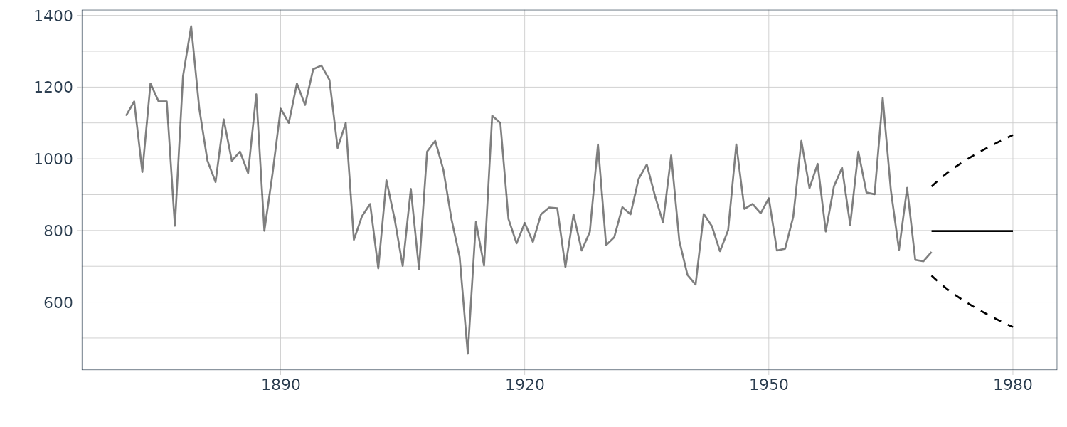
Kalman Smoothing
This book focuses on fixed-interval smoothing. Hence, we assume that Kalman filtering through time T has been completed before smoothing.
The smoothing distribution in the linear Gaussian state-space model is also the normal distribution. We define it as follows:
\[\begin{aligned} N(\textbf{s}_{t}, \textbf{S}_{t}) \end{aligned}\]The procedure for obtaining the smoothing distribution at time t from that at time \(t + 1\) is as follows:
Smoothing distribution at time \(t + 1\):
\[\begin{aligned} N(\textbf{s}_{t+1}, \textbf{S}_{t+1}) \end{aligned}\]Update procedure at time \(t\):
Smoothing gain:
\[\begin{aligned} \textbf{A}_{t} \leftarrow \textbf{C}_{t}\textbf{G}_{t+1}^{T}\textbf{R}_{t+1}^{-1} \end{aligned}\]State update:
\[\begin{aligned} \textbf{s}_{t} \leftarrow \textbf{m}_{t} + \textbf{A}_{t}[\textbf{s}_{t+1} - \textbf{a}_{t+1}]\\ \textbf{S}_{t} \leftarrow \textbf{C}_{t} + \textbf{A}_{t}[\textbf{S}_{t+1} - \textbf{R}_{t+1}]\textbf{A}_{t}^{T} \end{aligned}\]Smoothing distribution at time \(t\):
\[\begin{aligned} N(\textbf{s}_{t}, \textbf{S}_{t}) \end{aligned}\]Repeating the procedure of the above RTS (Rauch–Tung–Striebel) algorithm from \(t = T − 1\) in the reverse time direction, we obtain the smoothing distribution at every time point. Note that the smoothing distribution at time T corresponds to the filtering distribution at time T. The filtering distribution is corrected based on the smoothing distribution at one time point ahead.
t_max <- 100
# Function performing Kalman smoothing for one time point
Kalman_smoothing <- function(dat, s_t_plus_1, S_t_plus_1, t) {
  # Smoothing gain
  A_t <- dat$C[t] %*% t(G_t_plus_1) %*% solve(dat$R[t + 1])

  # State update
  s_t <- dat$m[t] + A_t %*% (s_t_plus_1 - dat$a[t + 1])
  S_t <- dat$C[t] + A_t %*% (S_t_plus_1 - dat$R[t + 1]) %*% t(A_t)

  # Return the mean and variance of the smoothing distribution
  return(
    list(
      s = s_t,
      S = S_t
    )
  )
}

# Find the mean and variance of the smoothing distribution

# Allocate memory for state (mean and covariance)
dat <- dat |>
  mutate(
    s = NA_real_,
    S = NA_real_
  )

# Time point: t = t_max
dat$s[t_max] <- dat$m[t_max]
dat$S[t_max] <- dat$C[t_max]

# Time point: t = t_max - 1 to 1
for (t in (t_max - 1):1) {
  KS <- Kalman_smoothing(dat, dat$s[t + 1], dat$S[t + 1], t = t)
  dat$s[t] <- KS$s
  dat$S[t] <- KS$S
}

# Ignore the display of following codes

# Find 2.5% and 97.5% values for 95% intervals
dat <- dat |>
  mutate(
    smooth_lower = s + qnorm(0.025, sd = sqrt(S)),
    smooth_upper = s + qnorm(0.975, sd = sqrt(S))
  )

dat |>
  autoplot(y, aes(color = "Obs")) +
  geom_line(aes(y = s, color = "Smooth")) +
  geom_ribbon(
    aes(
      ymax = smooth_upper,
      ymin = smooth_lower
    ),
    fill = "gray",
    alpha = 0.5
  ) +
  scale_color_manual(
    name = "",
    breaks = c("Obs", "Smooth"),
    values = c("Obs" = "black", "Smooth" = "blue")
  ) +
  xlab("") +
  ylab("") +
  theme_tq()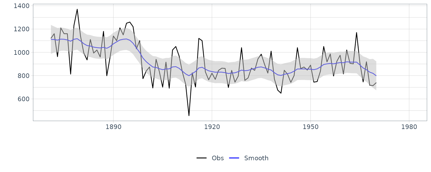
The code assumes that Kalman filtering has been completed. In the above code, we first define the function Kalman_smoothing(), which performs Kalman smoothing for one time point. For smoothing, we then use the function Kalman_smoothing() for every time point to obtain the mean and variance of the smoothing distribution.
We will now go through examples using the dlm library.
Example: Local-Level Model Case
The local-level model is defined as follows:
\[\begin{aligned} x_{t} &= x_{t-1} + w_{t}\\ y_{t} &= x_{t} + v_{t} \end{aligned}\] \[\begin{aligned} w_{t} &\sim N(0, W)\\ v_{t} &\sim N(0, V) \end{aligned}\]The above model corresponds to the linear Gaussian state-space model that has the settings:
\[\begin{aligned} p &= 1\\ \textbf{G}_{t} &= \begin{bmatrix} 1 \end{bmatrix}\\ \textbf{F}_{t} &= \begin{bmatrix} 1 \end{bmatrix} \end{aligned}\]Furthermore, for simplicity, we assume a time-invariant model:
\[\begin{aligned} W_{t} &= W\\ V_{t} &= V \end{aligned}\]The state equation for the local-level model states that the current observations are roughly the same as the previous ones and that there is no particular time pattern. The local-level model is similar to the AR(1) model with \(\phi = 1\). Such a coefficient leads to the nonstationary time series for the state known as a random walk. For this reason, the local-level model is also called a random walk plus noise model.
If there is no particular knowledge of a prior distribution, mean is set to an arbitrary finite value such as 0 or observations’ average, whereas variance is set to an arbitrary finite value such as a sufficiently large value according to the data. Even such a pragmatic policy does not cause a problem.
Using library dlm in R:
library(dlm)

mod <- dlmModPoly(order = 1)

> str(mod)
List of 10
 $ m0 : num 0
 $ C0 : num [1, 1] 1e+07
 $ FF : num [1, 1] 1
 $ V  : num [1, 1] 1
 $ GG : num [1, 1] 1
 $ W  : num [1, 1] 1
 $ JFF: NULL
 $ JV : NULL
 $ JGG: NULL
 $ JW : NULL
 - attr(*, "class")= chr "dlm"
We set order = 1 because the local-level model is generally a polynomial model of order one. The arguments dW and dV indicate the variances \(W\) and \(V\) of the state and observation noises, respectively. After the setting of the default value to them, they are updated to appropriate values through the specification of parameter values to be described later. The arguments m0 and C0 indicate the mean \(m_{0}\) and variance \(C_{0}\) of the prior distribution, respectively. While the default values 0 and \(10^{7}\) are set to them, the mean is finite and the variance is sufficiently larger than the data variance var(Nile) = 28,638. Hence, we need not update them.
The return values from dlmModPoly() are m0, C0, FF, V, GG, W, JFF, JV, JGG, and JW. In these elements, those with a name starting from J in the second half are used to specify the time-varying model. Since this example assumes the time-invariant local-level model, we need not change their settings from the default NULL.
The first-half elements m0, C0, FF, V, GG, and W correspond to:
\[\begin{aligned} \text{m}_{0}, \text{C}_{0}, \text{F}_{t}, V_{t}, \text{G}_{t}, \text{W}_{t} \end{aligned}\]When the model contains unknown parameters, we must specify their values in some manner for time series estimation. In this example, the parameters \(W, V\) are unknown and lack any specific clues. Hence we must specify these values. We attempt to use the maximum likelihood method because the data Nile are of a sufficient quantity.
build_dlm <- function(par) {

  mod$W[1, 1] <- exp(par[1])
  mod$V[1, 1] <- exp(par[2])

  return(mod)
}
The user-defined function build_dlm() is prepared for defining and building a model. Specifically, this function updates the unknown parameters \(W, V\) in mod by the values in argument par and returns the entire mod. Since both \(W, V\) are variances and do not take negative values, an exponential transformation is applied to par to ensure that the function optim() can avoid an unnecessary search of the negative region.
When the function build_dlm() references an object mod internally, R copies the mod internally and automatically.
fit_dlm <- dlmMLE(
  y = Nile,
  parm = c(0, 0),
  build = build_dlm,
  hessian = TRUE
)

> fit_dlm
$par
[1] 7.291951 9.622437

$value
[1] 549.6918

$counts
function gradient
      34       34

$convergence
[1] 0

$message
[1] "CONVERGENCE: REL_REDUCTION_OF_F <= FACTR*EPSMCH"

$hessian
         [,1]     [,2]
[1,] 2.096148  5.35176
[2,] 5.351760 36.70078
The argument parm is the initial searching values for the parameters in the maximum likelihood estimation and we can set the arbitrary finite value to those. The argument build is a user-defined function for defining and building a model. Regarding the algorithm performing the maximum likelihood estimation numerically, the L-BFGS method, a kind of quasi-Newton method, is used by default.
We can derive the standard error for each parameter in the maximum likelihood estimation from the Hessian matrix for the log-likelihood function. The Hessian matrix contains the second-order partial derivatives of a function as its elements. In this example, the log-likelihood function \(l()\) contains the parameters \(W, V\). Hence, the Hessian matrix is as follows:
\[\begin{aligned} H &= -\begin{bmatrix} \frac{\partial^{2}l(W, V)}{\partial W \partial W} & \frac{\partial^{2}l(W, V)}{\partial W \partial V}\\[5pt] \frac{\partial^{2}l(W, V)}{\partial V \partial W} & \frac{\partial^{2}l(W, V)}{\partial V \partial V} \end{bmatrix} \end{aligned}\]When we set the additional argument hessian = TRUE to the function dlmMLE(), it is passed through the function optim(), and the Hessian matrix evaluated at the minimum value of the negative log-likelihood is to be included in the return values. We are doing this because we are finding the maximum in MLE and not the minimum.
However, this example cannot use them directly because of the exponentially transformed parameters. Thus, we use the delta method to obtain the standard error of the parameters after exponential transformation:
\[\begin{aligned} \textrm{var}(e^{\theta}) &\approx \textrm{var}\Big(e^{\hat{\theta}} + \frac{e^{\hat{\theta}}}{1!}(\theta - \hat{\theta})\Big)\\ &= e^{2\hat{\theta}}\textrm{var}(\theta - \hat{\theta})\\ &= e^{2\hat{\theta}}\textrm{var}(\theta) \end{aligned}\]The diagonal elements of \(H^{-1}\) have \(\textrm{var}(\theta)\). Hence, we obtain the standard error of a parameter after exponential transformation as:
\[\begin{aligned} e^{\text{MLE Estimate}} \times \sqrt{\text{diag}(H^{-1})} \end{aligned}\]> exp(fit_dlm$par) * sqrt(diag(solve(fit_dlm$hessian)))
[1] 1280.170 3145.999Building the model with estimates from MLE:
mod <- build_dlm(fit_dlm$par)

> mod
$FF
     [,1]
[1,]    1

$V
        [,1]
[1,] 15099.8

$GG
     [,1]
[1,]    1

$W
         [,1]
[1,] 1468.432

$m0
[1] 0

$C0
      [,1]
[1,] 1e+07
Filtering in R:
dlmFiltered_obj <- dlmFilter(
  y = Nile,
  mod = mod
)

> str(dlmFiltered_obj, max.level = 1)
List of 9
 $ y  : Time-Series [1:100] from 1871 to 1970: 1120 1160 963 1210 1160 ...
 $ mod:List of 10
  ..- attr(*, "class")= chr "dlm"
 $ m  : Time-Series [1:101] from 1870 to 1970: 0 1118 1140 1072 1117 ...
 $ U.C:List of 101
 $ D.C: num [1:101, 1] 3162.3 122.8 88.9 76 70 ...
 $ a  : Time-Series [1:100] from 1871 to 1970: 0 1118 1140 1072 1117 ...
 $ U.R:List of 100
 $ D.R: num [1:100, 1] 3162.5 128.6 96.8 85.1 79.8 ...
 $ f  : Time-Series [1:100] from 1871 to 1970: 0 1118 1140 1072 1117 ...
 - attr(*, "class")= chr "dlmFiltered"
The return value from dlmFilter() is a list with the dlmFiltered class. The elements of the list are y, mod, m, U.C, D.C, a, U.R, D.R, and f.
The elements y, mod, m, U.C, D.C, a, U.R, D.R, and f correspond to:
- the input observations
- a list for model
- mean of filtering distribution
- two singular value decompositions for the covariance matrix of filtering distribution
- mean of one-step-ahead predictive distribution
- two singular value decompositions for the covariance matrix of one-step-ahead predictive distribution
- mean of one-step-ahead predictive likelihood
Since an object corresponding to the prior distribution is added at the beginning of m, U.C, and D.C, their length is one more than that of the observations.
dat <- as_tsibble(Nile)
dat <- dat |>
  rename(
    y = value
  ) |>
  mutate(
    m = dropFirst(dlmFiltered_obj$m),
    m_sdev = sqrt(
      dropFirst(
        as.numeric(
          dlmSvd2var(
            dlmFiltered_obj$U.C,
            dlmFiltered_obj$D.C
          )
        )
      )
    ),
    lower = m + qnorm(0.025, sd = m_sdev),
    upper = m + qnorm(0.975, sd = m_sdev)
  )
We drop a first element corresponding to the prior distribution in advance using the utility function dropFirst() of dlm. Since the covariance of the filtering distribution is decomposed into the elements U.C and D.C, we retrieve the original covariance matrix using the utility function dlmSvd2var() of dlm.
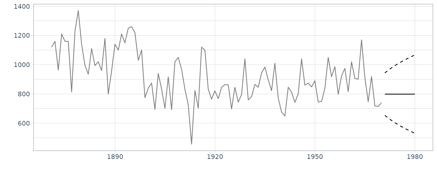
Predicting in R:
dlmForecasted_obj <- dlmForecast(
  mod = dlmFiltered_obj,
  nAhead = 10
)

# Confirmation of the results
> str(dlmForecasted_obj, max.level = 1)
List of 4
 $ a: Time-Series [1:10, 1] from 1971 to 1980: 798 798 798 798 798 ...
  ..- attr(*, "dimnames")=List of 2
 $ R:List of 10
 $ f: Time-Series [1:10, 1] from 1971 to 1980: 798 798 798 798 798 ...
  ..- attr(*, "dimnames")=List of 2
 $ Q:List of 10

dat_pred <- new_data(dat, n = nAhead)
dat_pred <- dat_pred |>
  mutate(
    a = dlmForecasted_obj$a,
    a_sdev = sqrt(
      as.numeric(
        dlmForecasted_obj$R
      )
    ),
    lower = a + qnorm(0.025, sd = a_sdev),
    upper = a + qnorm(0.975, sd = a_sdev)
  )
Smoothing in R:
dlmSmoothed_obj <- dlmSmooth(y = Nile, mod = mod)
> str(dlmSmoothed_obj, max.level = 1)
List of 3
$ s : Time-Series [1:101] from 1870 to 1970: 1111 1111 ...
$ U.S:List of 101
$ D.S: num [1:101, 1] 74.1 63.5 56.9 53.1 50.9 ...
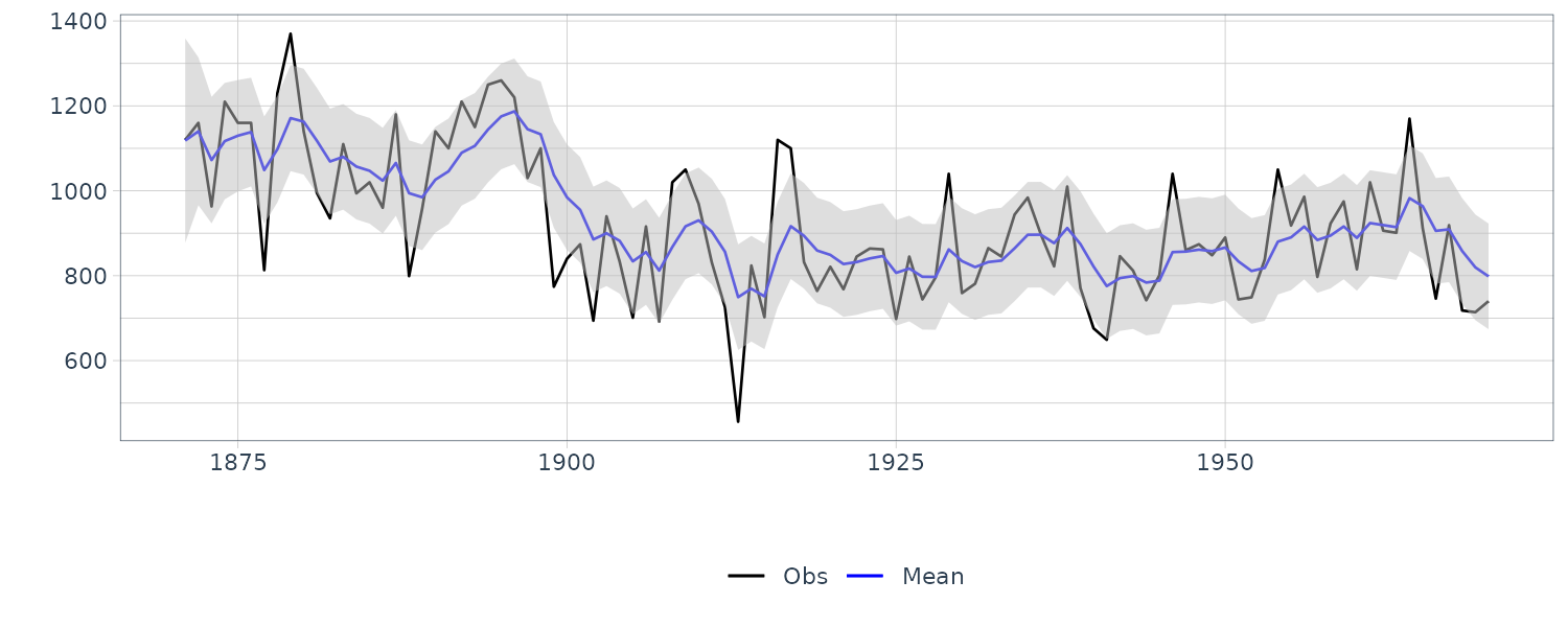
dat <- dat |>
mutate(
s = dropFirst(dlmSmoothed_obj$s),
s_sdev = sqrt(
dropFirst(
as.numeric(
dlmSvd2var(
dlmSmoothed_obj$U.S,
dlmSmoothed_obj$D.S
)
)
)
),
s_lower = s + qnorm(0.025, sd = s_sdev),
s_upper = s + qnorm(0.975, sd = s_sdev)
)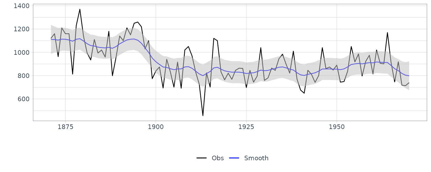
We see that the mean value and the probability intervals become smoother and more narrow, respectively. While the filtering is based on the past and current information, the smoothing can further consider the relative future information; it can generally improve the estimation accuracy. However, even smoothing cannot capture the sudden decrease in 1899. To capture such a situation adequately, we must incorporate particular information into the model we will introduce a method using a regression model later.
We now diagnose the model with innovations using the library dlm:
dat$residuals <- residuals(
object = dlmFiltered_obj,
sd = FALSE
)
dat |>
autoplot(residuals) +
ggtitle("Residuals") +
theme_tq()
dat |>
ACF(residuals) |>
autoplot() +
ggtitle("ACF") +
theme_tq()
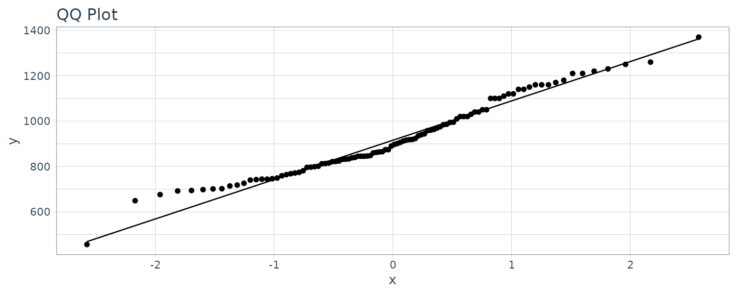
dat |>
ggplot(aes(sample = y)) +
ggtitle("QQ Plot") +
stat_qq() +
stat_qq_line() +
theme_tq()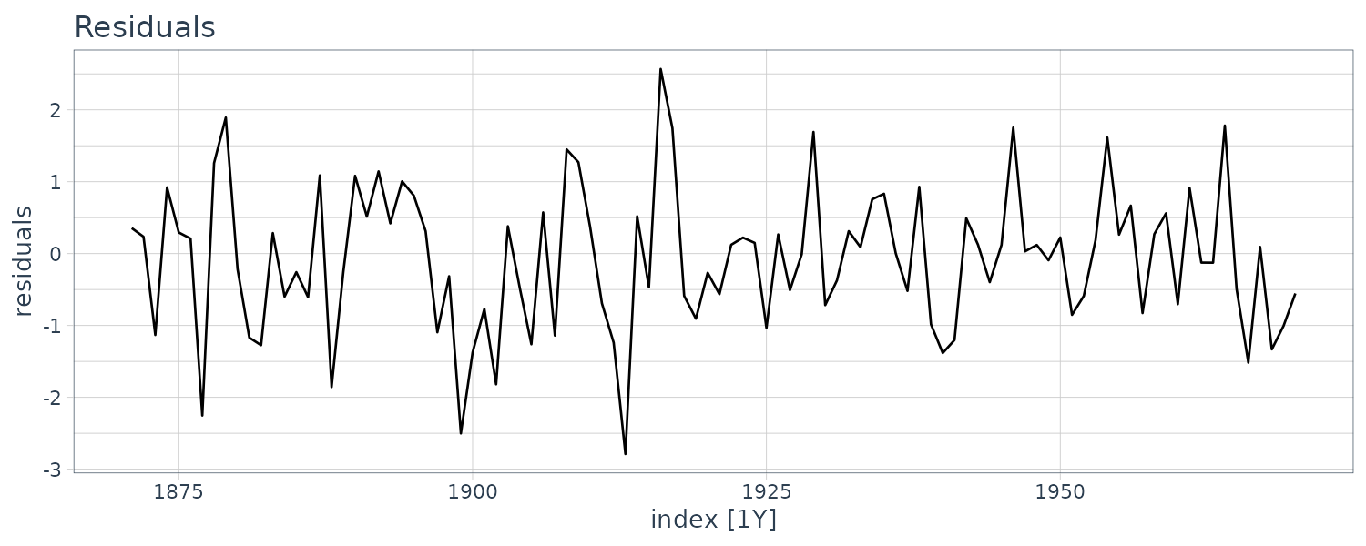

Local-Trend Model
A local-trend model is also known as a linear growth model and can express a linear slope in the data. Thus, this model is suitable for describing time series data with a trend of rising and falling for a particular term. The local-trend model is generally a polynomial model of order two.
We distinguish each element with a superscript(n) and refer to N as the order of the polynomial model. A state in the polynomial model comprises N elements:
\[\begin{aligned} \begin{bmatrix} x_{t}^{(N)}\\ \vdots\\ x_{t}^{(n)}\\ \vdots\\ x_{t}^{(1)} \end{bmatrix} \end{aligned}\]The state and observation equations for the polynomial model with time-invariant state and observation noises are as follows:
\[\begin{aligned} x_{t}^{(n)} &= x_{t-1}^{(n)} + x_{t-1}^{(n-1)} + w_{t}^{(n)} \end{aligned}\] \[\begin{aligned} w_{t}^{(n)} &\sim N(0, W^{(n)}) \end{aligned}\] \[\begin{aligned} n &= N, \cdots, 2\\[10pt] \end{aligned}\] \[\begin{aligned} x_{t}^{(1)} &= x_{t-1}^{(1)} + w_{t}^{(1)} \end{aligned}\] \[\begin{aligned} w_{t}^{(1)} &\sim N(0, W^{(1)})\\[10pt] \end{aligned}\] \[\begin{aligned} y_{t} &= x_{t}^{(N)} + v_{t} \end{aligned}\] \[\begin{aligned} v_{t} &\sim N(0, V)\\[10pt] \end{aligned}\] \[\begin{aligned} \mathbf{x}_{t} &= \begin{bmatrix} x_{t}^{(N)}\\ \vdots\\ x_{t}^{(2)}\\ x_{t}^{(1)} \end{bmatrix} \end{aligned}\]Setting \(w_{t}^{(n)} = 0\) reveals the relation:
\[\begin{aligned} x_{t}^{(n)} - x_{t-1}^{(n)} &= x_{t-1}^{(n-1)} \end{aligned}\]Based on this property, \(x_{t}^{(N)}\) is interpreted as the level for short term. \(x_{t}^{(N-1)} = x_{t}^{(N)} - x_{t-1}^{(N)}\) is interpreted as the slope for short term. And \(x_{t}^{(N-2)} = x_{t}^{(N-1)} - x_{t-1}^{(N-1)}\) is interpreted as the curvature for short term, etc. Polynomial models of the order N = 3 and more are not generally used because with an increase in N, the estimation result overfits the noise and becomes difficult to interpret.
\[\begin{aligned} \mathbf{G}_{t} &= \begin{bmatrix} 1 & 1 & & &\\ & 1 & 1& &\\ & & \ddots & \ddots &\\ & & & 1&1\\ 0 & 0 & \cdots & 0&1\\ \end{bmatrix} \end{aligned}\] \[\begin{aligned} \mathbf{W}_{t} &= \begin{bmatrix} W^{(N)} & & &\\ &\ddots & &\\ & & W^{(2)}&\\ & & &W^{(1)}\\ \end{bmatrix} \end{aligned}\] \[\begin{aligned} \mathbf{F}_{t} &= \begin{bmatrix} 1 & 0 & \cdots & 0 \end{bmatrix} \end{aligned}\] \[\begin{aligned} V_{t} &= V \end{aligned}\]The polynomial model with the setting \(W^{(N)} = \cdots = W^{(2)} = 0\) is particularly referred to the integrated random walk model. Incidentally, this model is equivalent to taking the N-th difference of the data at preprocessing. We can recognize that the integrated random walk model in the state-space model corresponds to the difference at preprocessing in the ARIMA model.
The example of the local-trend model is illustrated with the seasonal model in the next section.
Seasonal Model
The seasonal model is also known as periodical model and is suitable for expressing a model that has a clear periodic pattern in the observations. This section explains two approaches for defining the model: time domain and frequency domain approaches.
Approach from the Time Domain
Let the cycle be s and the seasonal component be \(x_{t}\). Then, such a property is expressed as follows:
\[\begin{aligned} \sum_{t=1}^{s}x_{t} &= \text{any constant that does not differ from the sum in another cycle} \end{aligned}\]The constant can be considered as 0. When we assume that such a fluctuation has a normal distribution with mean 0, the equation becomes as follows:
\[\begin{aligned} \sum_{t=1}^{s}x_{t} &= w_{t} \end{aligned}\] \[\begin{aligned} w_{t} &\sim N(0, W) \end{aligned}\]This equation imposes a constraint on the seasonality.
Next, as a specific explanation, consider the data with quarter seasonality. Let the seasonal component at time point t be:
\[\begin{aligned} \begin{bmatrix} x_{t-4}\\ x_{t-3}\\ x_{t-2}\\ x_{t-1} \end{bmatrix} &= \begin{bmatrix} x_{t-1}^{(4Q)}\\ x_{t-1}^{(1Q)}\\ x_{t-1}^{(2Q)}\\ x_{t-1}^{(3Q)} \end{bmatrix} \end{aligned}\]The time transitions of these elements are expressed as follows:
\[\begin{aligned} x_{t}^{(1Q)} \leftarrow x_{t-1}^{(4Q)}\\ x_{t}^{(2Q)} \leftarrow x_{t-1}^{(1Q)}\\ x_{t}^{(3Q)} \leftarrow x_{t-1}^{(2Q)}\\ x_{t}^{(4Q)} \leftarrow x_{t-1}^{(3Q)} \end{aligned}\]Recalling that the value of 4Q can be defined by those of 1Q, 2Q, and 3Q from the constraint. We can further reduce the above equations. The right-hand side can be rewritten with the values of 1Q, 2Q, and 3Q:
\[\begin{aligned} x_{t}^{(1Q)} &\leftarrow -x_{t-1}^{(1Q)} -x_{t-1}^{(2Q)} -x_{t-1}^{(3Q)} + w_{t}\\ x_{t}^{(2Q)} &\leftarrow x_{t-1}^{(1Q)}\\ x_{t}^{(3Q)} &\leftarrow x_{t-1}^{(2Q)}\\ \end{aligned}\]Finally, we generally define the state and observation equations based on the above descriptions. The state and observation equations for the seasonal model in the time-domain approach, with time-invariant state and observation noises:
\[\begin{aligned} \textbf{x}_{t} &= \begin{bmatrix} x_{t}^{(1)}\\ x_{t}^{(2)}\\ \vdots\\ x_{t}^{(s-1)} \end{bmatrix} \end{aligned}\] \[\begin{aligned} \textbf{G}_{t} &= \begin{bmatrix} -1 & \cdots & -1 & -1\\ 1 & & &\\ & \ddots & &\\ & & 1 & \end{bmatrix} \end{aligned}\] \[\begin{aligned} \textbf{W}_{t} &= \begin{bmatrix} W & & &\\ & 0 & &\\ & & \ddots &\\ & & &0 \end{bmatrix} \end{aligned}\] \[\begin{aligned} \textbf{F}_{t} &= \begin{bmatrix} 1 & 0 & \cdots &0 \end{bmatrix} \end{aligned}\] \[\begin{aligned} V_{t} &= V \end{aligned}\]Approach from the Frequency Domain
This approach is based on Fourier series expansion and can easily adjust the number \(N\) of frequency components to be considered. While there are various kinds of seasonalities, the gradual seasonality can lead to a more natural interpretation than the complicated one in many cases, and the former is further able to suppress the overfitting to the noise. The setting low \(N\) in this model can achieve such a gradual seasonality and even sometimes improve the marginal likelihood as a result.
Arbitrary periodic data can generally be represented by the infinite sum of its frequency components.
Let the periodic real-valued signal be \(\gamma_{t}\). Its complex-valued Fourier series can be expressed as follows:
\[\begin{aligned} \gamma_{t} &= \sum_{n=-\infty}^{\infty}c_{n}e^{in\omega_{0}t}\\ &= c_{0} + \sum_{n=1}^{\infty}\bar{c}_{n}e^{-in\omega_{0}t} + \sum_{n=1}^{\infty}c_{n}e^{in\omega_{0}t} \end{aligned}\] \[\begin{aligned} \omega_{0} &= \frac{2\pi}{s} \end{aligned}\]Where \(\omega_{0}\) is the fundamental angular frequency and s is the (fundamental) period. For example, for a 12-month seasonal, the fundamental period \(s = 12\).
The first term is a component with frequency 0, i.e., no periodicity, implying an offset for the entire periodic signal. This term is often treated with a polynomial model in the state-space model and can be ignored.
The second and third terms contribute to the negative and positive frequency components, respectively, and negative and positive frequencies abstractly imply clockwise and counterclockwise rotations, respectively. If we treat the real-valued periodic signals in the state-space model, we can ignore either of them because the second and third terms have a complex conjugate relationship. This relation makes the imaginary part of real-valued signal \(\gamma_{t}\) become zero. Thus, if the observation matrix doubles the real part (in-phase component) and neglects the imaginary part (quadrature-phase component) of either term, the other becomes unnecessary.
We decide here to ignore the third term, contributing to the positive frequency component. In addition, while the Fourier series is generally an infinite sum, if and only if the period s is a rational number, it can be represented by a finite sum through \(\left \lfloor{\frac{s}{2}}\right \rfloor\) from the sampling theorem.
In accordance with the above description, we redefine the fourier series equation with a finite sum of only negative frequency components as follows:
\[\begin{aligned} \gamma_{t} &\equiv \sum_{n=1}^{N}2\bar{c}_{n}e^{-in\omega t}\\ &= \sum_{n=1}^{N}\gamma_{t}^{(n)} \end{aligned}\] \[\begin{aligned} \gamma_{t}^{(n)} &= 2\bar{c}_{n}e^{-in\omega t} \end{aligned}\]Next, considering the time transition of \(\gamma_{t}^{(n)}\), we have:
\[\begin{aligned} \gamma_{t+1}^{(n)} =\ &2\bar{c}_{n}e^{-in\omega_{0}(t+1)}\\ =\ &2\bar{c}_{n}e^{-in\omega_{0}t}e^{-in\omega_{0}}\\ =\ &\gamma_{t}^{(n)}e^{-in\omega_{0}}\\ =\ &\Big(\text{Re}(\gamma_{t}^{(n)}) + i\text{Im}(\gamma_{t}^{(n)})\Big)\Big(\textrm{cos}(n\omega_{0}) - i\ \textrm{sin}(n\omega_{0})\Big)\\ =\ &\Big(\text{Re}(\gamma_{t}^{(n)})\textrm{cos}(n\omega_{0}) + \textrm{Im}(\gamma_{t}^{(n)})\textrm{sin}(n\omega_{0})\Big)\\ &+\ i\Big(-\text{Re}(\gamma_{t}^{(n)})\textrm{sin}(n\omega_{0}) + \textrm{Im}(\gamma_{t}^{(n)})\textrm{cos}(n\omega_{0})\Big) \end{aligned}\]We can rewrite the above equation by representing the real and imaginary part as elements of the vector:
\[\begin{aligned} \begin{bmatrix} \text{Re}(\gamma_{t+1}^{(n)})\\ \text{Im}(\gamma_{t+1}^{(n)}) \end{bmatrix} &= \begin{bmatrix} \text{cos}(n\omega_{0}) & \text{sin}(n\omega_{0})\\ -\text{sin}(n\omega_{0}) & \text{cos}(n\omega_{0}) \end{bmatrix} \begin{bmatrix} \text{Re}(\gamma_{t}^{(n)})\\ \text{Im}(\gamma_{t}^{(n)}) \end{bmatrix}\\ &= \text{rotation matrix}^{(n)}\begin{bmatrix} \text{Re}(\gamma_{t}^{(n)})\\ \text{Im}(\gamma_{t}^{(n)}) \end{bmatrix} \end{aligned}\]We see that this is a state equation wherein the state for each frequency component is represented by:
\[\begin{aligned} \begin{bmatrix} \text{Re}(\gamma_{t}^{(n)})\\ \text{Im}(\gamma_{t}^{(n)}) \end{bmatrix} \end{aligned}\]However, the state noise is not yet considered. Note that we ignore \(\text{Im}(\gamma_{t}^{(n)})\) eventually and assign \(\text{Re}(\gamma_{t}^{(n)})\) only to the observations.
Finally, we define the state and observation equations generally based on the above descriptions. The state and observation equations for the seasonal model in the frequency-domain approach with time-invariant state and observation noises with the following settings:
\[\begin{aligned} \textbf{x}_{t} &= \begin{bmatrix} \textrm{Re}(y_{t}^{(1)})\\ \textrm{Im}(y_{t}^{(1)})\\ \textrm{Re}(y_{t}^{(2)})\\ \textrm{Im}(y_{t}^{(2)})\\ \vdots\\ \textrm{Re}(y_{t}^{(N-1)})\\ \textrm{Im}(y_{t}^{(N-1)})\\ \textrm{Re}(y_{t}^{(N)})\\ \textrm{Im}(y_{t}^{(N)})\\ \end{bmatrix} \end{aligned}\] \[\begin{aligned} \textbf{G}_{t} &= \begin{bmatrix} \text{rotation matrix}^{(1)} & & & &\\ & \text{rotation matrix}^{(2)}& & &\\ &&\ddots&&\\ &&&\text{rotation matrix}^{(N-1)}&\\ &&&&\text{rotation matrix}^{(N)}\\ \end{bmatrix} \end{aligned}\] \[\begin{aligned} \textbf{W}_{t} &= \begin{bmatrix} W^{(1)}&&&&&&&&\\ &W^{(1)}&&&&&&&\\ &&W^{(2)}&&&&&&\\ &&&W^{(2)}&&&&&\\ &&&&\ddots&&&&\\ &&&&&W^{(N-1)}&&&\\ &&&&&&W^{(N-1)}&&\\ &&&&&&&W^{(N)}&\\ &&&&&&&&W^{(N)} \end{bmatrix} \end{aligned}\] \[\begin{aligned} \textbf{F}_{t} &= \begin{bmatrix} 1 & 0 & 1 & 0 & \cdots & 1 & 0 & 1 & 0 \end{bmatrix} \end{aligned}\] \[\begin{aligned} V_{t} &= V \end{aligned}\] \[\begin{aligned} \omega_{0} &= \frac{2\pi}{s} \end{aligned}\]Example: CO2 Concentration in the Atmosphere
Now, we analyze CO2 concentration data in the atmosphere, using the linear Gaussian state-space model. As noted in Sect. 4.3, these data show an annual seasonality and an increasing trend. We apply a combination of the local-trend and seasonal models. Based on this decision, we compare three model variations.
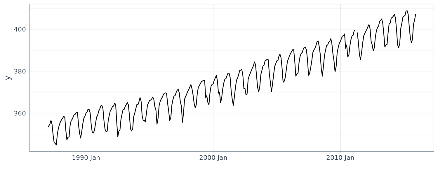
Local-Trend Model + Seasonal Model (Time-Domain Approach)
This case uses the seasonal model with the time-domain approach. We can achieve such a model through the following setting in the component decomposition.
The state and observation equations of the local-trend model with time-invariant state and observation noises are as follows:
\[\begin{aligned} \textbf{x}_{t} &= \begin{bmatrix} x_{t}^{(2)}\\ x_{t}^{(1)} \end{bmatrix} \end{aligned}\] \[\begin{aligned} \textbf{G}_{t} &= \begin{bmatrix} 1 & 1\\ 0 & 1 \end{bmatrix} \end{aligned}\] \[\begin{aligned} \textbf{F}_{t} &= \begin{bmatrix} 1 & 0 \end{bmatrix} \end{aligned}\] \[\begin{aligned} \textbf{W}_{t} &= \begin{bmatrix} W^{(2)} & 0\\ 0 & W^{(1)} \end{bmatrix} \end{aligned}\] \[\begin{aligned} V_{t} &= V \end{aligned}\]And the state and observation equations of the season models:
\[\begin{aligned} \textbf{x}_{t} &= \begin{bmatrix} \textbf{x}_{t}^{(1)}\\ \textbf{x}_{t}^{(2)}\\ \vdots\\ \textbf{x}_{t}^{(11)} \end{bmatrix} \end{aligned}\] \[\begin{aligned} \textbf{G}_{t} &= \begin{bmatrix} -1 & \cdots & -1 & -1\\ 1 & & &\\ & \ddots & &\\ & & 1 & \end{bmatrix} \end{aligned}\] \[\begin{aligned} \textbf{W}_{t} &= \begin{bmatrix} \textbf{W}_{t} & & &\\ & 0 & &\\ & & \ddots &\\ & & & 0 \end{bmatrix} \end{aligned}\] \[\begin{aligned} \textbf{F}_{t} &= \begin{bmatrix} 1 & 0 & \cdots & 0 \end{bmatrix} \end{aligned}\] \[\begin{aligned} V_{t} &= V \end{aligned}\]build_dlm_CO2a <- function(par) {
return(
dlmModPoly(
order = 2,
dW = exp(par[1:2]),
dV = exp(par[3])
) +
dlmModSeas(
frequency = 12,
dW = c(
exp(par[4]),
rep(0, times = 10)
),
dV = 0
)
)
}
fit_dlm_CO2a <- dlmMLE(
y = dat$y,
parm = rep(0, 4),
build = build_dlm_CO2a
)
> fit_dlm_CO2a
$par
[1] -2.4760362 -23.4799981 -0.1567843 -4.4814964
$value
[1] 336.4054
$counts
function gradient
46 46
$convergence
[1] 0
$message
[1] "CONVERGENCE: REL_REDUCTION_OF_F <= FACTR*EPSMCH"
mod <- build_dlm_CO2a(fit_dlm_CO2a$par)
> str(mod, max.level = 1)
List of 10
$ m0 : num [1:13] 0 0 0 0 0 0 0 0 0 0 ...
$ C0 : num [1:13, 1:13] 10000000 0 0 0 0 0 0 0 0 0 ...
$ FF : num [1, 1:13] 1 0 1 0 0 0 0 0 0 0 ...
$ V : num [1, 1] 0.855
$ GG : num [1:13, 1:13] 1 0 0 0 0 0 0 0 0 0 ...
$ W : num [1:13, 1:13] 0.0841 0 0 0 0 ...
$ JFF: NULL
$ JV : NULL
$ JGG: NULL
$ JW : NULL
- attr(*, "class")= chr "dlm"Kalman filtering:
dlmFiltered_obj <- dlmFilter(
  y = dat$y,
  mod = mod
)

mu <- dropFirst(dlmFiltered_obj$m[, 1])
gamma <- dropFirst(dlmFiltered_obj$m[, 3])

dat <- dat |>
  mutate(
    mu = dropFirst(dlmFiltered_obj$m[, 1]),
    gamma = dropFirst(dlmFiltered_obj$m[, 3])
  )

dat1 <- dat |>
  slice(100:n())

plot_grid(
  dat1 |>
    autoplot(y) +
    theme_tq(),
  dat1 |>
    autoplot(mu) +
    theme_tq(),
  dat1 |>
    autoplot(gamma) +
    theme_tq(),
  ncol = 1
)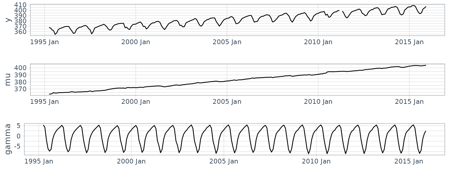
The arguments dW and dV indicate the diagonal elements \(W^{(2)}, W^{(1)}\) in the covariance of the state noise and variance \(V\) of the observation noise, respectively. These are respectively set to exp(par[1:2]) and exp(par[3]) based on the argument par of build_dlm_CO2a().
The arguments m0 and C0 are set to the default values, i.e., 0 and \(10^{7}\textbf{I}\), respectively.
The function dlmModSeas() sets the seasonal model in the time-domain approach. The arguments of this function are frequency, dW, dV, m0, and C0. The argument frequency indicates the period s; hence, we set frequency = 12 as the annual cycle. The arguments dW and dV indicate the diagonal elements \(W, 0, \cdots, 0\) in the covariance of the state noise and variance V of the observation noise, respectively. The argument dW is set to c(exp(par[4]), rep(0, times = 10)) based on the argument par of build_dlm_CO2a().
From the level and seasonal components, we understand that the estimation accuracy for the first year deteriorates because the mean vector of the prior distribution is set to 0 and consistency with the data are not particularly considered. Such a situation can be mitigated through mean vector refinement of the prior distribution or Kalman smoothing.
Local-Trend Model + Seasonal Model (Frequency-Domain Approach)
The following equations are applied to the second component model:
\[\begin{aligned} \textbf{x}_{t} &= \begin{bmatrix} \textrm{Re}(y_{t}^{(1)})\\ \textrm{Im}(y_{t}^{(1)})\\ \textrm{Re}(y_{t}^{(2)})\\ \textrm{Im}(y_{t}^{(2)}) \end{bmatrix} \end{aligned}\] \[\begin{aligned} \textbf{G}_{t} &= \begin{bmatrix} \text{rotation matrix}^{(1)} &\\ & \text{rotation matrix}^{(2)} \end{bmatrix} \end{aligned}\] \[\begin{aligned} \textbf{W}_{t} &= \begin{bmatrix} W^{(1)}&&&\\ &W^{(1)}&&\\ &&W^{(2)}&\\ &&&W^{(2)} \end{bmatrix} \end{aligned}\] \[\begin{aligned} \textbf{F}_{t} &= \begin{bmatrix} 1 & 0 & 1 & 0 \end{bmatrix} \end{aligned}\] \[\begin{aligned} V_{t} &= V \end{aligned}\] \[\begin{aligned} \omega_{0} &= \frac{2\pi}{s} \end{aligned}\]build_dlm_CO2c <- function(par) {
return(
dlmModPoly(
order = 2,
dW = exp(par[1:2]),
dV = exp(par[3])
) +
dlmModTrig(
s = 12,
q = 2,
dW = exp(par[4]),
dV = 0
)
)
}
fit_dlm_CO2c <- dlmMLE(
y = dat$y,
parm = rep(0, 4),
build = build_dlm_CO2c
)
fit_dlm_CO2c
mod <- build_dlm_CO2c(fit_dlm_CO2c$par)
# Kalman filtering
dlmFiltered_obj <- dlmFilter(y = dat$y, mod = mod)
dat <- dat |>
mutate(
mu = dropFirst(dlmFiltered_obj$m[, 1]),
gamma = dropFirst(
dlmFiltered_obj$m[, 3] + dlmFiltered_obj$m[, 5]
)
)
dat1 <- dat |>
slice(100:n())
plot_grid(
dat1 |>
autoplot(y) +
theme_tq(),
dat1 |>
autoplot(mu) +
theme_tq(),
dat1 |>
autoplot(gamma) +
theme_tq(),
ncol = 1
)
The arguments of dlmModTrig function are s, q, dV, dW, m0, C0, om, and tau. This example does not use om and tau because they are set when the fundamental period s is not an integer.
The argument s indicates the fundamental period s, which is an integer in this example, and we set s = 12 as the annual cycle. The argument q indicates the value N of the number of frequency components we leave in order from the low frequency. Such a value must be optimized, and this example sets 2 as the optimum value.
The arguments dW and dV indicate the diagonal elements in the covariance of the state noise and the variance V of the observation noise, respectively. The seasonal model in the frequency-domain approach can set the variance of the state noise individually as \(W^{(1)}, \cdots, W^{(N)}\) for each frequency component. However, if there is no particular prior information, we typically set the unique value W to them. Since there are also no specific informations in this example, dW is set to exp(par[4]) as a unique value. The argument dV has already been set through dlmModPoly(), hence we set 0 here.
And doing a prediction in R:
nAhead <- 12
dlmForecasted_object <- dlmForecast(
  mod = dlmFiltered_obj,
  nAhead = nAhead
)

dat_pred <- new_data(dat, n = nAhead)
dat_pred <- dat_pred |>
  mutate(
    f = dlmForecasted_object$f,
    f_sd = sqrt(as.numeric(dlmForecasted_object$Q)),
    lower = f + qnorm(0.025, sd = f_sd),
    upper = f + qnorm(0.975, sd = f_sd)
  )

dat |>
  slice(300:n()) |>
  autoplot(y, alpha = 0.5) +
  geom_line(
    aes(y = f),
    data = dat_pred
  ) +
  geom_line(
    aes(y = upper),
    linetype = "dashed",
    data = dat_pred
  ) +
  geom_line(
    aes(y = lower),
    linetype = "dashed",
    data = dat_pred
  ) +
  xlab("") +
  ylab("") +
  theme_tq()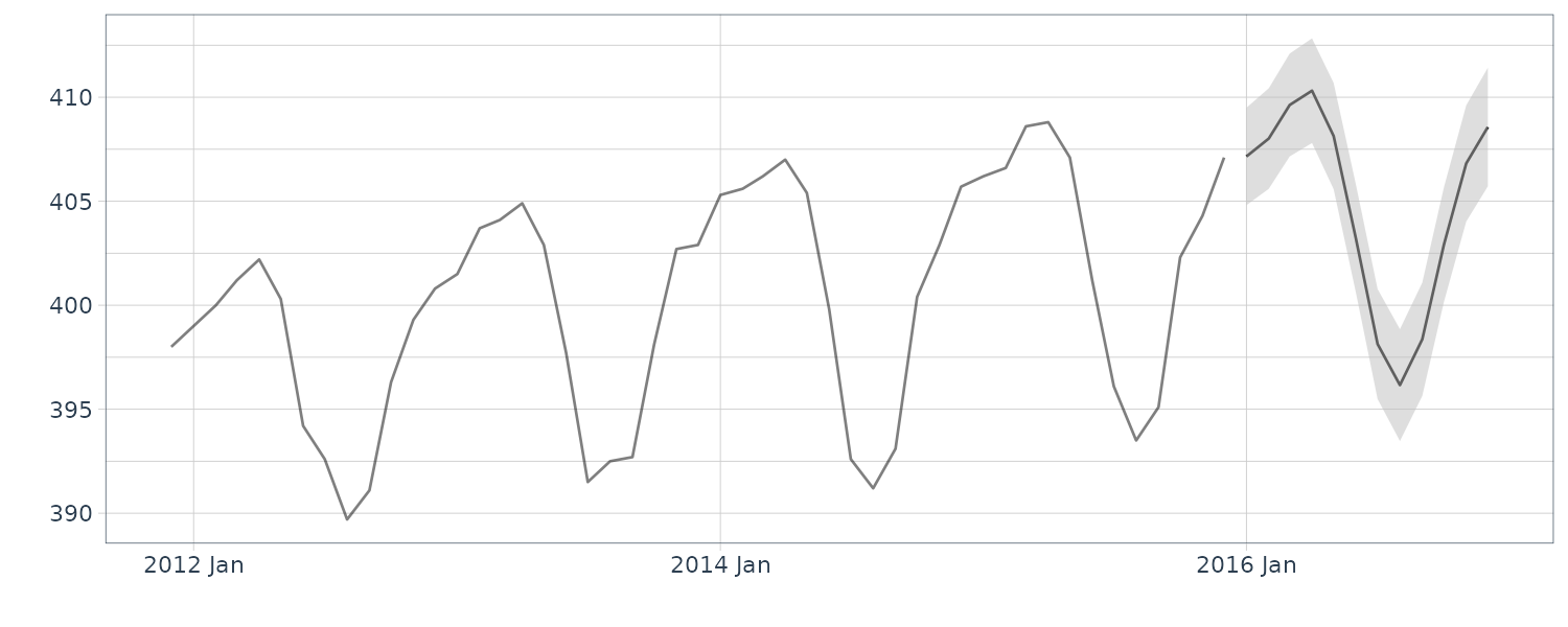
It is worth noting that the model a) uses 11 states to express seasonality, whereas the model c) uses only 4 states. The number 11 is derived from the “12-month period − constraint on the time domain period,” and the number 4 is also derived from “two artificially set residual frequency components × each real and imaginary part”.
ARMA Model
The ARMA model can be defined as an individual model in the state-space model. If the original time series data are nonstationary, we sometimes take the multiple-times difference of the data to achieve stationarity before applying the ARMA model. Such a model is called the ARIMA model. In the state-space model, we typically apply the polynomial and seasonal models to the nonstationary components.
In the state-space model, it is common to treat the correlation between data by primarily combining the polynomial and seasonal models introduced thus far. However, with actual data, irregular fluctuations can remain even with such a combinational model for various reasons.
For example, unexpected events may not be fully explained by such a model. In the state-space model, the ARMA model is effective in capturing and expressing such residual correlation. We typically use a low-order stationary AR model for this purpose.
We now consider the below expression in the state-space model:
\[\begin{aligned} y_{t} &= \sum_{j=1}^{r}\phi_{j}y_{t-j} + \sum_{j=1}^{r-1}\theta_{j}e_{t-j} + e_{t} \end{aligned}\] \[\begin{aligned} r &= \textrm{max}(p, q + 1) \end{aligned}\] \[\begin{aligned} \phi_{j} &= 0, j > p \end{aligned}\] \[\begin{aligned} \theta_{j} &= 0, j > q \end{aligned}\]While there are several expressions of ARMA model with state-space form, this book uses the observable canonical form. The state and observation equations for the ARMA model with the following settings:
\[\begin{aligned} \textbf{x}_{t} &= \begin{bmatrix} x_{t}^{(1)}\\ x_{t}^{(2)}\\ \vdots\\ x_{t}^{(r-1)}\\ x_{t}^{(r)} \end{bmatrix} \end{aligned}\] \[\begin{aligned} \textbf{G}_{t} &= \begin{bmatrix} \phi_{1} & 1 & & &\\ \phi_{2} & & 1 & &\\ \vdots & & &\ddots &\\ \phi_{r-1} & & & & 1\\ \phi_{r} & 0& 0& \cdots& 0\\ \end{bmatrix} \end{aligned}\] \[\begin{aligned} \textbf{W}_{t} &= \textbf{R}\textbf{R}^{T}\sigma^{2} \end{aligned}\] \[\begin{aligned} \textbf{R} &= \begin{bmatrix} 1\\ \theta_{1}\\ \vdots\\ \theta_{r-2}\\ \theta_{r-1}\\ \end{bmatrix} \end{aligned}\] \[\begin{aligned} \textbf{F}_{t} &= \begin{bmatrix} 1 & 0 & \cdots & 0 & 0 \end{bmatrix} \end{aligned}\] \[\begin{aligned} V_{t} &= 0 \end{aligned}\]Note that the above setting leads to:
\[\begin{aligned} \textbf{w}_{t} &= \textbf{R}e_{t} \end{aligned}\]The state equation is expanded as:
\[\begin{aligned} x_{t}^{(1)} &= \phi_{1}x_{t-1}^{(1)} + x_{t-1}^{(2)} + e_{t}\\ x_{t}^{(2)} &= \phi_{2}x_{t-1}^{(1)} + x_{t-1}^{(3)} + \theta_{1}e_{t}\\ &\ \ \vdots\\ x_{t}^{(r-1)} &= \phi_{r-1}x_{t-1}^{(1)} + x_{t-1}^{(r)} + \theta_{r-2}e_{t}\\ x_{t}^{(r)} &= \phi_{r}x_{t-1}^{(1)} + \theta_{r-1}e_{t}\\ \end{aligned}\]Subsituting successively we get:
\[\begin{aligned} x_{t}^{(1)} &= \phi_{1}x_{t-1}^{(1)} + \phi_{2}x_{t-2}^{(1)} + x_{t-2}^{(3)} + \theta_{1}e_{t-1} + e_{t}\\ &\ \ \vdots\\ &= \phi_{1}x_{t-1}^{(1)} + \cdots + \phi_{r}x_{t-r}^{(1)}+ \theta_{1}e_{t-1} + \cdots + \theta_{r-1}e_{t-(r-1)} + e_{t} \end{aligned}\]Lastly, the observation equation \(y_{t} = x_{t}^{(1)}\) yields:
\[\begin{aligned} y_{t} &= \phi_{1}y_{t-1} + \cdots + \phi_{r}y_{t-r} + \theta_{1}e_{t-1} + \cdots + \theta_{r-1}e_{t-(r-1)} + e_{t} \end{aligned}\]Example: Japanese Beer Production
We analyze the data on Japanese beer production. Plotting the dataset in R:
beer <- read.csv("BEER.csv")

beer <- beer |>
  mutate(
    y = Shipping_Volume,
    log_y = log(y),
    t = yearmonth(
      paste0(
        substr(Year_Month, 1, 4),
        "-",
        substr(Year_Month, 5, 6)
      )
    )
  ) |>
  as_tsibble(index = t)

beer |>
  autoplot(y) +
  xlab("") +
  scale_y_continuous(labels = scales::comma) +
  theme_tq()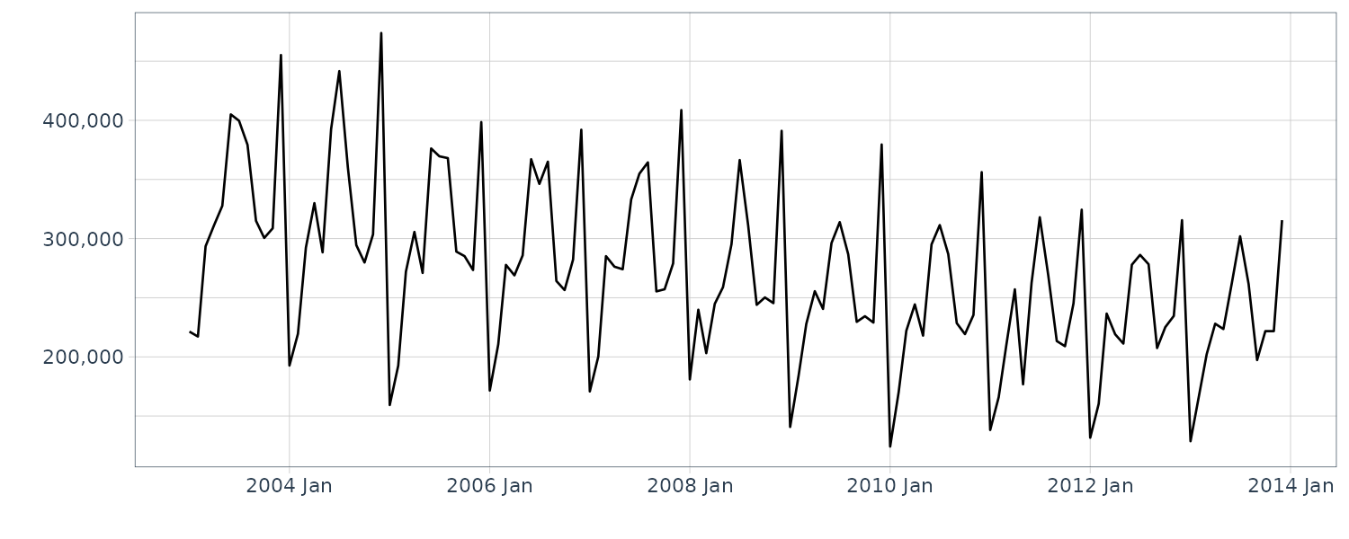
The range of data fluctuation appears to decrease with increasing time. It is known empirically that such economic data often show an exponential tendency. Thus, we decide to apply the logarithmic transformation.
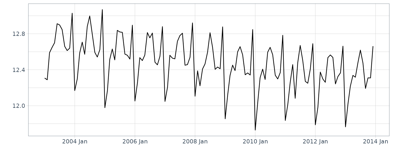
We also see the annual cycle and decreasing trend for the essential characteristics of the time series. The annual cycle arises from the beer demand, which tends to increase in the summer and at the end of the year. In addition, the decreasing trend can be affected by young people’s lack of interest in beer.
Then, we consider the model to be applied. First, we model the annual cycle. The cycle has extremely sharp changes; such a change in the time domain corresponds to the high-frequency component in the frequency domain. Seasonality can be modeled using two approaches (time and frequency domains). The frequency-domain approach appears not to have any advantage in this example because the data originally have high-frequency components that must not be truncated. Thus, we decide to use the seasonal model in the time-domain approach. Its state elements are more intuitive and easier to understand.
Local-Level Model + Seasonal Model (Time-Domain Approach)
In R:
build_dlm_BEERb <- function(par) {
  return(
    dlmModPoly(
      order = 1,
      dW = exp(par[1]),
      dV = exp(par[2])
    ) +
      dlmModSeas(
        frequency = 12,
        dW = c(
          exp(par[3]),
          rep(0, times = 10)
        ),
        dV = 0
      )
  )
}

fit_dlm_BEERb <- dlmMLE(
  y = beer$y,
  parm = rep(0, 3),
  build = build_dlm_BEERb
)

mod <- build_dlm_BEERb(fit_dlm_BEERb$par)

dlmSmoothed_obj <- dlmSmooth(
  y = beer$y,
  mod = mod
)

beer <- beer |>
  mutate(
    mu = dropFirst(dlmSmoothed_obj$s[, 1]),
    gamma = dropFirst(dlmSmoothed_obj$s[, 3])
  )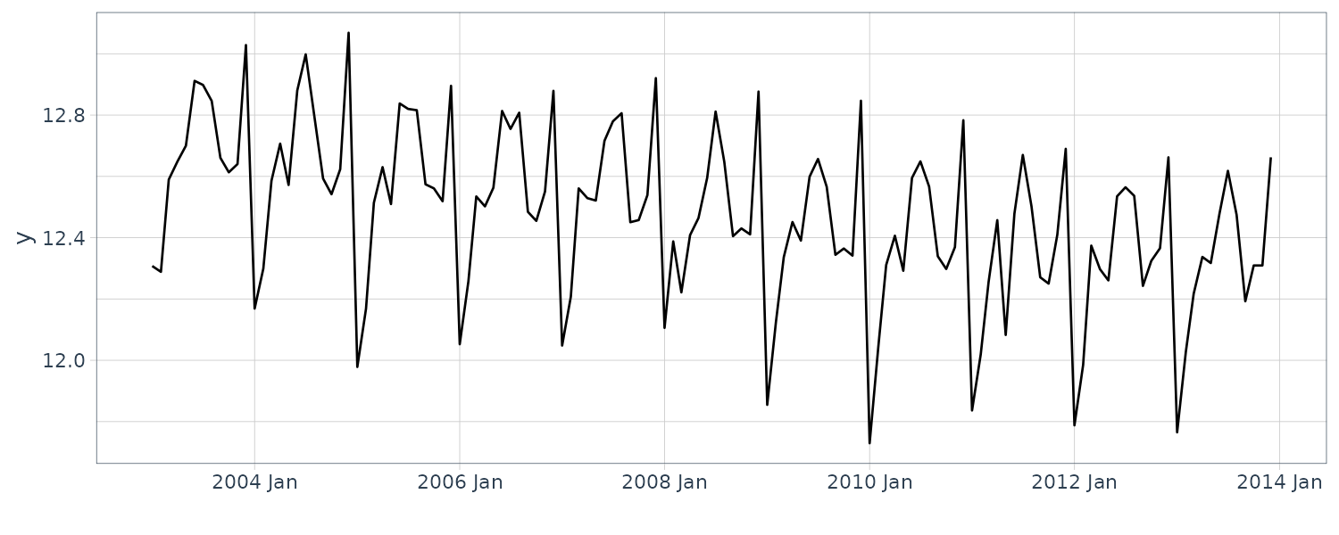
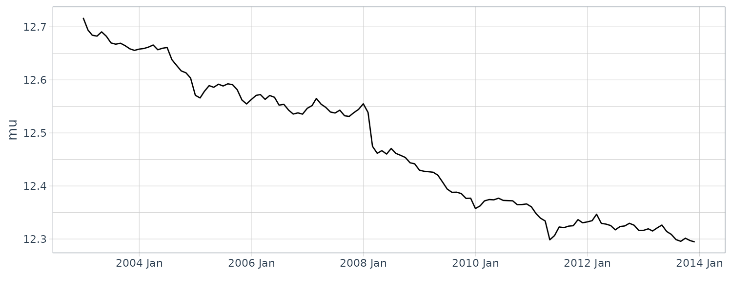
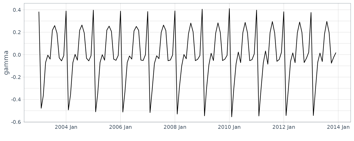
Local-Level Model + Seasonal Model (Time-Domain Approach) + ARMA Model
We try improving the result further by adding the ARMA model. The ARMA model captures the residual correlations due to various factors working together: adult population, price revision, weather, tax, economy, competing products, and natural disasters.
For simplicity, we decide here to use the purest AR(1) model to capture the irregular deviation from the supposed smoothing level. We will use the following for the 3rd component model:
\[\begin{aligned} \textbf{x}_{t} &= \begin{bmatrix} x_{t}^{(1)} \end{bmatrix} \end{aligned}\] \[\begin{aligned} \textbf{G}_{t} &= \begin{bmatrix} \phi_{1} \end{bmatrix} \end{aligned}\] \[\begin{aligned} \textbf{W}_{t} &= \sigma^{2} \end{aligned}\] \[\begin{aligned} \textbf{R} &= \begin{bmatrix} 1 \end{aligned}\] \[\begin{aligned} \textbf{F}_{t} &= \begin{bmatrix} 1 \end{bmatrix} \end{aligned}\] \[\begin{aligned} V_{t} &= 0 \end{aligned}\]In R:
build_dlm_BEERc <- function(par) {
  return(
    dlmModPoly(
      order = 1,
      dW = exp(par[1]),
      dV = exp(par[2])
    ) +
      dlmModSeas(
        frequency = 12,
        dW = c(
          exp(par[3]),
          rep(0, 10)
        ),
        dV = 0
      ) +
      dlmModARMA(
        ar = ARtransPars(par[4]),
        sigma2 = exp(par[5])
      )
  )
}

fit_dlm_BEERc <- dlmMLE(
  y = beer$y,
  parm = rep(0, 5),
  build = build_dlm_BEERc
)

> fit_dlm_BEERc
$par
[1] -8.816820e+00 -6.100818e+00 -9.465262e+00
[4] -4.884259e-05 -6.922353e+00

$value
[1] -152.6774

$counts
function gradient
      90       90

$convergence
[1] 0

$message
[1] "CONVERGENCE: REL_REDUCTION_OF_F <= FACTR*EPSMCH"

> ARtransPars(fit_dlm_BEERc$par[4])
[1] -4.884259e-05

mod <- build_dlm_BEERc(fit_dlm_BEERc$par)

dlmSmoothed_obj <- dlmSmooth(
  y = beer$y,
  mod = mod
)

beer <- beer |>
  mutate(
    mu = dropFirst(dlmSmoothed_obj$s[, 1]),
    gamma = dropFirst(dlmSmoothed_obj$s[, 2]),
    arma = dropFirst(dlmSmoothed_obj$s[, 13])
  )
The arguments of dlmModARMA() are ar, ma, sigma2, dV, m0, and C0. The argument ar indicates the AR coefficient \(\phi_{j}\) and must be specified preserving stationarity. For such a purpose, the library dlm provides a utility function ARtransPars() that approximates the AR coefficients.
The argument ma indicates the MA coefficient \(\theta_{j}\). Because this example does not use it, the default value NULL is applied. The argument sigma2 indicates the variance \(\sigma^{2}\) of the white noise and is set to exp(par[5]) based on the argument par of build_dlm_BEERc().
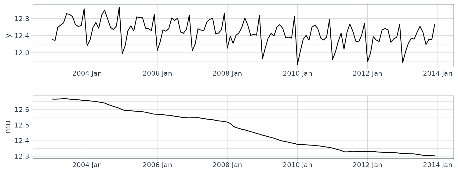
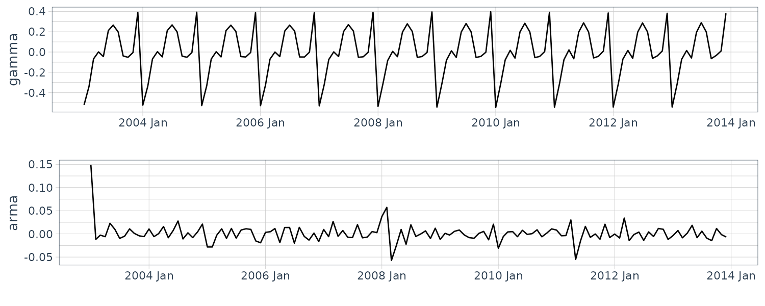
The AR(1) component reflects irregular distortion. Specifically, the significant distortion of the AR(1) component at the beginning of 2008 is hypothesized to be rush demand and its backlash, which are associated with the price rise implemented at that time. However, we cannot determine the causality easily.
In the above example, the AR(1) coefficient takes a small value. This result indicates that the ARMA model captures fine distortion. On the other hand, if the AR(1) coefficient takes a greater value, then the ARMA model can capture rough distortion. The ARMA model is often used for the latter purpose.
Regression Model
The regression model is used to enhance the explanation capability of the model by considering the relation with the event, which might be useful for describing time series data. We call the value quantifying such an event by some means an explanatory variable, such as temperature, population, or an indicator of 0/1 showing the occurrence or nonoccurrence of an event (this is also called an intervention variable).
The state-space model also considers the regression component as one of the individual models:
\[\begin{aligned} y_{t} &= \alpha_{t} + \beta_{1t}x_{1t} + \cdots + \beta_{nt}x_{nt} + \cdots + \beta_{Nt}x_{Nt} + v_{t} \end{aligned}\]We assume that all of these variables can change over time. The regression intercept \(\alpha_{t}\) and coefficient \(\beta_{nt}\) are stochastic and must be estimated, while the explanatory variable \(x_{nt}\) is deterministic.
\[\begin{aligned} \textbf{x}_{t} &= \begin{bmatrix} \alpha_{t}\\ \beta_{1t}\\ \vdots\\ \beta_{Nt} \end{bmatrix} \end{aligned}\] \[\begin{aligned} \textbf{G}_{t} &= \textbf{I} \end{aligned}\] \[\begin{aligned} \textbf{W}_{t} &= \begin{bmatrix} W^{(\alpha)} & & &\\ & W^{(1)} & & \\ & & \ddots& \\ & & & W^{(N)} \end{bmatrix} \end{aligned}\] \[\begin{aligned} \textbf{F}_{t} &= \begin{bmatrix} 1 & x_{1t} & \cdots & x_{Nt} \end{bmatrix} \end{aligned}\] \[\begin{aligned} V_{t} &= V \end{aligned}\]The above dynamic linear regression model estimates the time-varying regression intercept and coefficient. This is the advantage of this model and differs from standard static linear regression. The setting \(\textbf{W}_{t} = \textbf{0}\) eliminates the temporal transition of the regression intercept and coefficient and renders the above model a standard static linear regression model.
Example: Nintendo’s Stock Price
We now examine the beta value for Nintendo’s stock price. The beta value is an index showing how the individual stock price changes aggressively compared to the market average. We proceed with the analysis based on a single regression model supposing that Nintendo’s stock price, the Nikkei stock average, and the beta correspond to the observations, an explanatory variable, and a regression coefficient, respectively.
The following component decomposition applied to the first component model:
\[\begin{aligned} \textbf{x}_{t} &= \begin{bmatrix} \alpha_{t}\\ \beta_{1t} \end{bmatrix} \end{aligned}\] \[\begin{aligned} \textbf{G}_{t} &= \textbf{I} \end{aligned}\] \[\begin{aligned} \textbf{W}_{t} &= \begin{bmatrix} W^{(\alpha)} &\\ & W^{(1)} \end{bmatrix} \end{aligned}\] \[\begin{aligned} \textbf{F}_{t} &= \begin{bmatrix} 1 & x_{1t} \end{bmatrix} \end{aligned}\] \[\begin{aligned} V_{t} &= V \end{aligned}\]build_dlm_REG <- function(par) {
dlmModReg(
X = dat$nikkei,
dW = exp(par[1:2]),
dV = exp(par[3])
)
}
fit_dlm_REG <- dlmMLE(
y = dat$Close,
parm = rep(0, 3),
build = build_dlm_REG
)
> fit_dlm_REG
$par
[1] 2.765568e-07 -5.186491e+00 -7.071863e-07
$value
[1] 1233.212
$counts
function gradient
9 9
$convergence
[1] 0
$message
[1] "CONVERGENCE: REL_REDUCTION_OF_F <= FACTR*EPSMCH"
mod <- build_dlm_REG(fit_dlm_REG$par)
> str(mod)
List of 11
$ m0 : num [1:2] 0 0
$ C0 : num [1:2, 1:2] 1e+07 0e+00 0e+00 1e+07
$ FF : num [1, 1:2] 1 1
$ V : num [1, 1] 1
$ GG : num [1:2, 1:2] 1 0 0 1
$ W : num [1:2, 1:2] 1 0 0 0.00559
$ JFF: num [1, 1:2] 0 1
$ JV : NULL
$ JGG: NULL
$ JW : NULL
$ X : num [1:160, 1] 14405 14562 14088 14202 14087 ...
- attr(*, "class")= chr "dlm"
dlmSmoothed_obj <- dlmSmooth(
y = dat$Close,
mod = mod
)
dat <- dat |>
mutate(
beta = dropFirst(dlmSmoothed_obj$s[, 2]),
beta_sdev = sqrt(
dropFirst(
sapply(
dlmSvd2var(
dlmSmoothed_obj$U.S,
dlmSmoothed_obj$D.S
), function(x) {
diag(x)[2]
}
)
)
),
lower = beta + qnorm(0.025, sd = beta_sdev),
upper = beta + qnorm(0.975, sd = beta_sdev)
)The arguments of dlmModReg() are X, addInt, dW, dV, m0, and C0. The argument X indicates a vector of explanatory variables \(x_{nt}\). The argument addInt indicates whether we are to include the regression intercept, and the default value TRUE is applied to it because this example considers the intercept. The arguments dW and dV indicate the diagonal elements \(W^{(\alpha)}, W^{(1)}, \cdots, W^{(N)}\) in the covariance of the state noise and the variance V of the observation noise, respectively. We respectively set exp(par[1:2]) and exp(par[3]) to them based on the argument par of build_dlm_REG().
We find the elements $JFF and $X that have not been set in the former models. These elements are used for the time-varying model, and we see that the regression model has a time-varying parameter \(\textbf{F}_{t}\). So far we have assumed that the parameters in the stochastic model are time-invariant but the regression model is an exception in having time-varying parameters.
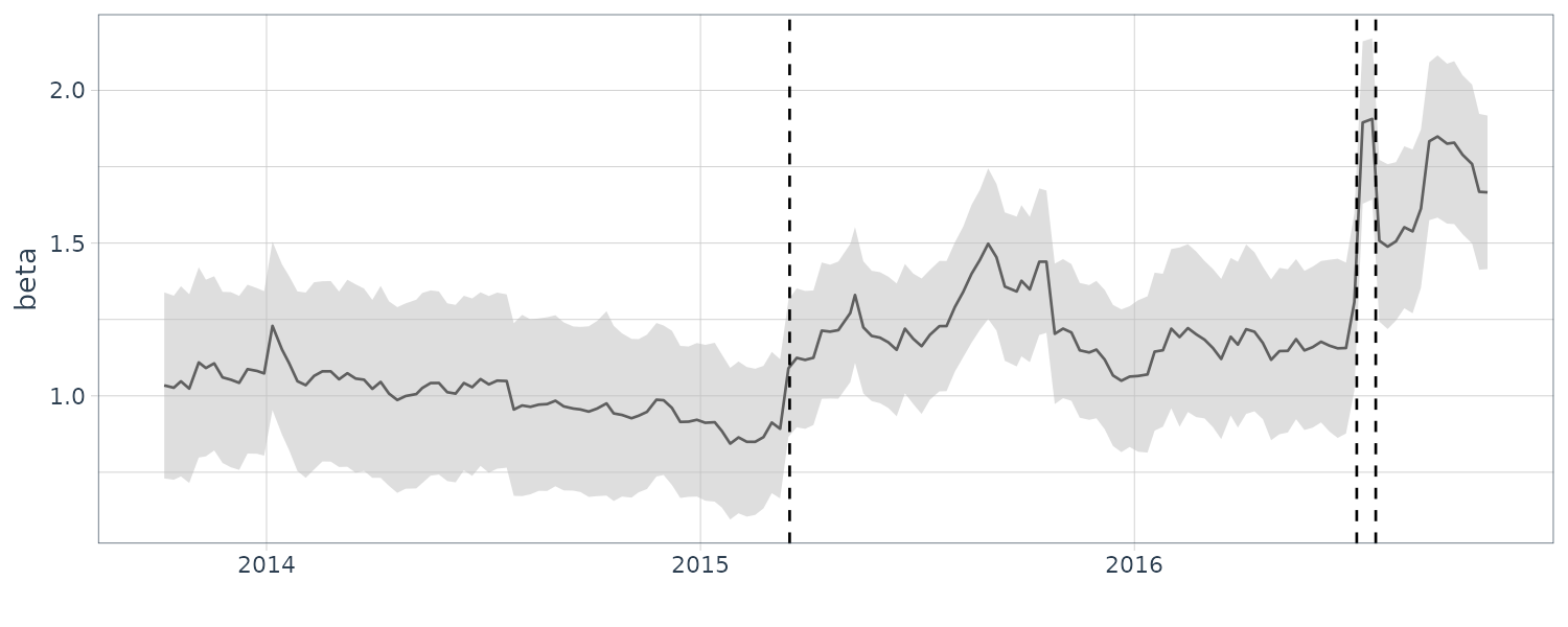
According to the plot, we see that the beta in this example looks basically like its stock price. The significant events related to Nintendo:
- March 17, 2015: Notice regarding business and capital alliance with DeNA Co., Ltd.
- July 6, 2016: Mobile game “Pokémon GO” launched in Australia, New Zealand, and the United States.
- July 22, 2016: Notice regarding the impact of “Pokémon GO” on the consolidated financial forecast.
The above events appear to affect the beta. However, since we cannot determine the causality easily.
Example: Flow Data of the Nile (Considering the Rapid Decrease in 1899)
While we have analyzed these data based on the state-space model, we could not capture adequately the rapid decrease in 1899. Although a simple means such as data division might be sufficient for these data, we attempt here to extend the model to capture structural changes even without such a division. For this purpose, we use the regression model to consider the rapid decrease in 1899.
Specifically, in the regression model, we set an explanatory variable to zero through 1899, that is, without a dam, and one after 1899, i.e., with a dam. An explanatory variable indicating the presence or absence of such an event is sometimes referred to as an intervention variable. We consider a model that contains such a regression component as well as the local-level component.
library(dlm)
set.seed(123)

dat <- Nile |>
  as_tsibble() |>
  rename(
    y = value
  )

t_max <- nrow(dat)

x_dash <- rep(0, t_max)
x_dash[dat$index >= 1899] <- 1

build_dlm_DAM <- function(par) {
  return(
    dlmModPoly(
      order = 1,
      dV = exp(par[1]),
      dW = exp(par[2])
    ) +
      dlmModReg(
        X = x_dash,
        addInt = FALSE,
        dW = exp(par[3]),
        dV = 0
      )
  )
}

fit_dlm_DAM <- dlmMLE(
  y = dat$y,
  parm = rep(0, 3),
  build = build_dlm_DAM
)
modtv <- build_dlm_DAM(fit_dlm_DAM$par)

> modtv
$FF
     [,1] [,2]
[1,]    1    1

$V
         [,1]
[1,] 16300.98

$GG
     [,1] [,2]
[1,]    1    0
[2,]    0    1

$W
             [,1]         [,2]
[1,] 0.0001422043 0.0000000000
[2,] 0.0000000000 0.0001989114

$JFF
     [,1] [,2]
[1,]    0    1

$X
     [,1]
[1,] 0
[2,] 0
[3,] ...

$m0
[1] 0 0

$C0
         [,1]     [,2]
[1,] 10000000        0
[2,]        0 10000000
First we do Kalman Filtering:
dlmFiltered_obj <- dlmFilter(
  y = dat$y,
  mod = modtv
)

modtv$V

mtv <- dropFirst(dlmFiltered_obj$m)
mtv_var <- dlmSvd2var(
  dlmFiltered_obj$U.C,
  dlmFiltered_obj$D.C
)
mtv_var <- mtv_var[-1]

coeff <- cbind(1, x_dash)
s_sdev <- sqrt(
  sapply(
    seq_along(stv_var),
    function(ct) {
      coeff[ct, ] %*%
        stv_var[[ct]] %*%
        t(coeff[ct, , drop = FALSE])
    }
  )
)
Next Kalman smoothing:
dlmSmoothed_obj <- dlmSmooth(
  y = dat$y,
  mod = modtv
)
stv <- dropFirst(dlmSmoothed_obj$s)
stv_var <- dlmSvd2var(
  dlmSmoothed_obj$U.S,
  dlmSmoothed_obj$D.S
)

stv_var <- stv_var[-1]

coeff <- cbind(1, x_dash)
s_sdev <- sqrt(
  sapply(
    seq_along(stv_var),
    function(ct) {
      coeff[ct, ] %*%
        stv_var[[ct]] %*%
        t(coeff[ct, , drop = FALSE])
    }
  )
)

# Mean for estimator
dat <- dat |>
  mutate(
    s = stv[, 1] + x_dash * stv[, 2],
    lower = s + qnorm(0.025, sd = s_sdev),
    upper = s + qnorm(0.975, sd = s_sdev)
  )
The function dlmModReg() in the library dlm sets the regression model. The argument X of this function is set to x_dash. In addition, the regression intercept is not used in this example; hence, the argument addInt is set to FALSE. The argument dW is set to exp(par[3]) based on the argument par of build_dlm_DAM(). Since the argument dV has already been set through the local-level model, we set 0 here.
The estimator in this model is the sum of two random variables, that is, the level + regression components; hence, we calculate its mean and variance based on:
\[\begin{aligned} E[X + Y] &= E[X] + E[Y] \end{aligned}\] \[\begin{aligned} \text{var}(X + Y) &= \text{var}(X) + \text{var}(Y) + 2E[(X - E[X])(Y - E[Y])] \end{aligned}\]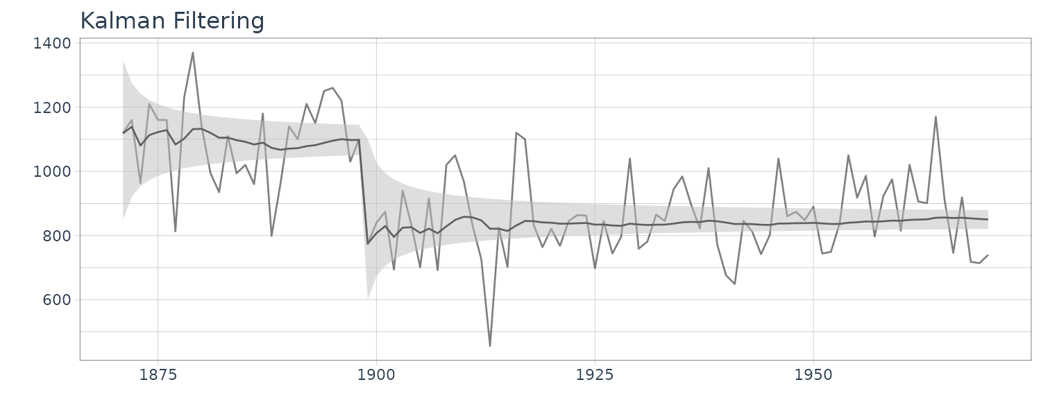
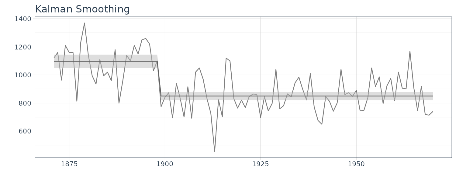
Example: Family Food Expenditure (Considering Effects Depending on the Days of the Week)
We now examine family food expenditures in Japan. The expenditure on food expenses is a continuous occurrence and affected by various factors such as prices and the economy.
In R:
food <- read.csv("FOOD.csv")

food <- food |>
  mutate(
    t = yearmonth(paste(Year, "-", Month))
  ) |>
  rename(
    y = Expenditure
  ) |>
  as_tsibble(index = t)
dat <- food |>
  mutate(
    y = log(y)
  )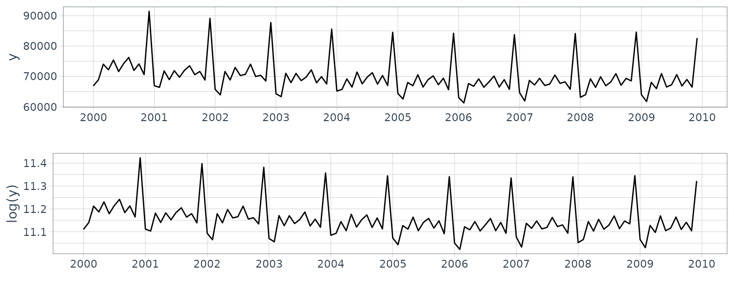
The level appears to be saturated after a moderate decreasing trend, except for the annual cycle. We also see that the annual cycle has the remarkable property of being the highest in December and the lowest in January or February. This property is the same as that of beer production; we can guess that both are influenced by Japanese culture.
We first apply the local-trend model to the entire decreasing trend. As for the annual cycle, we apply the seasonal model with the time-domain approach considering the sharp change between the year-end and new year similarly to beer production.
build_dlm_FOODa <- function(par) {
  return(
    dlmModPoly(
      order = 1,
      dW = exp(par[1]),
      dV = exp(par[2])
    ) +
      dlmModSeas(
        frequency = 12,
        dW = c(
          exp(par[3]),
          rep(0, times = 10)
        ),
        dV = 0
      )
  )
}

fit_dlm_FOODa <- dlmMLE(
  y = dat$y,
  parm = rep(0, 3),
  build = build_dlm_FOODa
)

mod <- build_dlm_FOODa(fit_dlm_FOODa$par)

> -dlmLL(y = dat$y, mod = mod)
[1] 312.291

dlmSmoothed_obj <- dlmSmooth(
  y = dat$y,
  mod = mod
)

dat <- dat |>
  mutate(
    mu = dropFirst(dlmSmoothed_obj$s[, 1]),
    gamma = dropFirst(dlmSmoothed_obj$s[, 3])
  )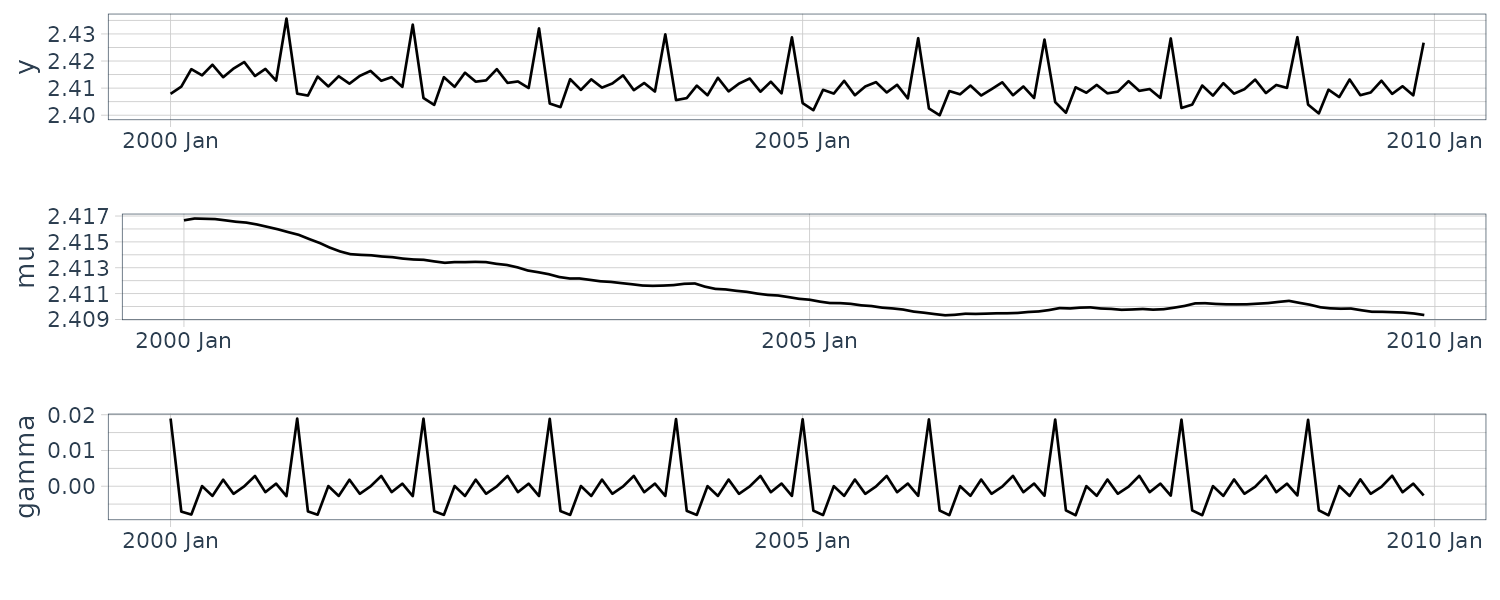
While this result provides a reasonable impression, we focus on the influence of the day of the week for further improvement. If the food expenditure did not change depending on the day of the week, we would not have to take such an effect into account. However, if the food expenditure considerably changes depending on the day of the week, we should consider such an effect because the total number of “day of the week” in one month varies according to the month, e.g., the number of Mondays may vary in different months.
Graphing the daily food expenditure of June 2009:
food_day <- read.csv("FOOD_DAY.csv")
food_day$t <- as.Date(food_day$Date)

food_day <- food_day |>
  rename(
    y = Expenditure
  ) |>
  as_tsibble(index = t)

food_day |>
  autoplot(y) +
  geom_vline(
    xintercept = food_day |>
      filter(wday(t) %in% c(6, 7)) |>
      pull(t),
    linetype = "dashed",
  ) +
  xlab("") +
  theme_tq()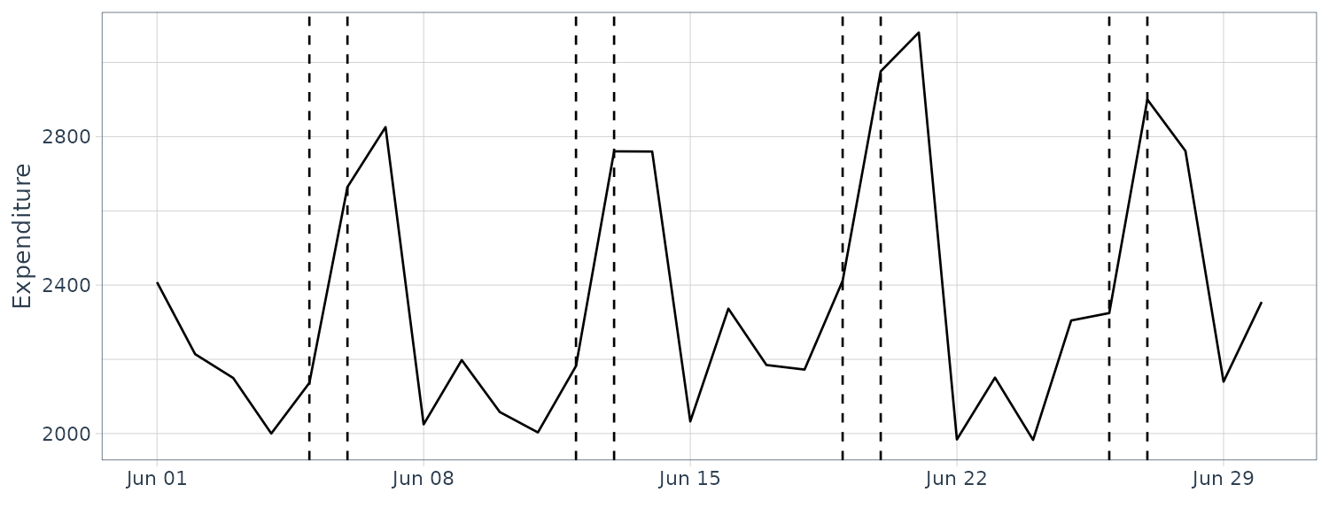
We find that the values on Saturdays and Sundays are significantly higher than those on other days. If we regard Saturdays and Sundays as typical holidays, we can suppose that food is inclined to be purchased on holidays intensively. Based on this assumption, we can expect that the national holidays also have the same inclination, while there are no national holidays in June 2009.
The above influence is called a calendar effect, and the state-space model can take its impact into account through the regression component, whose explanatory variable is set to the deterministic calendar information. While there are various means for the setting of such information, for monthly data, an explanatory variable is typically set to the monthly total number for each day of the week. This is often referred to as a trading-day effect:
\[\begin{aligned} \text{trading-day effect} = &\beta_{1} \times \text{monthly total number for the weekdays}\\ &+ \beta_{2} \times \text{monthly total number for the holidays}\\ \end{aligned}\]We assume time-invariant regression coefficients in the above effect because time-invariant coefficients result in static regression, which is easily interpreted and typically used. Furthermore, we assume that the sum of regression coefficients is zero to ensure the unique time series decomposition. Specifically, this example supposes the following constraint:
\[\begin{aligned} \beta_{1} + \beta_{2} &= 0 \end{aligned}\]Hence:
\[\begin{aligned} \text{trading-day effect} = &\ \beta_{1} \times (\text{monthly total number for the weekdays}\\ &- \text{monthly total number for the holidays})\\ \end{aligned}\]Thus, the trading-day effect in this example has an explanatory variable, “the number of weekdays more than holidays in one month”. Hereafter, we call this effect a “weekday effect”. The code setting the explanatory variable for this weekday effect is as follows:
jholidays <- function(days) {
  library(Nippon)

  DOW <- wday(days)

  holidays <- (DOW %in% c(6, 7)) | is.jholiday(days)

  # Overwrite the day of the week with "HOLIDAY" or "WEEKDAY"
  DOW[holidays] <- "Holiday"
  DOW[!holidays] <- "Weekday"

  return(DOW)
}

days <- seq(
  from = as.Date("2000/1/1"),
  to = as.Date("2009/12/31"),
  by = "day"
)

monthly <- table(
  substr(days, start = 1, stop = 7),
  jholidays(days)
)

x_dash_weekday <- monthly[, "Weekday"] - monthly[, "Holiday"]

t_max <- length(dat$y)

LEAPYEAR_FEB <- (c(2000, 2004, 2008) - 2000) * 12 + 2

x_dash_leapyear <- rep(0, t_max) # All initial value 0s
x_dash_leapyear[LEAPYEAR_FEB] <- 1

dat <- dat |>
  mutate(
    leapyear = rep(0, t_max),
    weekday = x_dash_weekday
  )
dat$leapyear[LEAPYEAR_FEB] <- 1
We add the regression model described above to the first discussed model, that is, the local-trend model + seasonal model (time-domain approach). Here, we simplify the first model in advance, because we expect that the regression model is to capture fine fluctuations residing in the observations. Specifically, we replace the local-trend model by the local-level model and set the state noise of the seasonal model in the time-domain approach to zero:
build_dlm_FOODb <- function(par) {
  return(
    dlmModPoly(
      order = 1,
      dW = exp(par[1]),
      dV = exp(par[2])
    ) +
      dlmModSeas(
        frequency = 12,
        dW = c(0, rep(0, times = 10)),
        dV = 0
      ) +
      dlmModReg(
        X = dat |>
          as_tibble() |>
          select(leapyear, weekday),
        addInt = FALSE,
        dV = 0
      )
  )
}

fit_dlm_FOODb <- dlmMLE(
  y = dat$y,
  parm = rep(0, 2),
  build = build_dlm_FOODb
)

mod <- build_dlm_FOODb(fit_dlm_FOODb$par)

> -dlmLL(y = dat$y, mod = mod)
[1] 193.3762

dlmSmoothed_obj <- dlmSmooth(
  y = dat$y,
  mod = mod
)

dat <- dat |>
  mutate(
    mu = dropFirst(dlmSmoothed_obj$s[, 1]),
    gamma = dropFirst(dlmSmoothed_obj$s[, 3])
  )

# Time-invariant. All the values are the same
beta_w <- dropFirst(dlmSmoothed_obj$s[, 13])[t_max]
beta_l <- dropFirst(dlmSmoothed_obj$s[, 14])[t_max]

> beta_w
[1] 0.03959524

> beta_l
[1] -0.001740371

# Mean of regression component
dat <- dat |>
  mutate(
    reg = dat |>
      as_tibble() |>
      select(leapyear, weekday) |>
      as.matrix() %*%
      c(beta_w, beta_l)
  )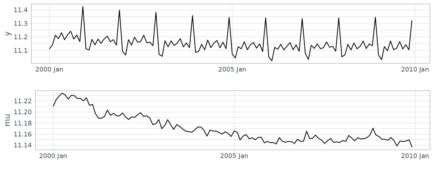
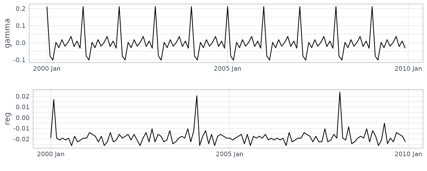
We find that the regression component grows in February of the leap year. Regarding the regression coefficients, we can obtain the rational values consistent with our assumption: the coefficient beta_w of the weekday effect takes the negative value −0.003098287, which indicates that the expenditure on weekdays decreases compared with that on holidays, while the coefficient beta_l of the leap-year effect takes the value 0.03920194, approximately 1/30, which indicates one day in a month.
Monte Carlo Markov Chain (MCMC)
In case of the linear Gaussian state-space model, we can derive its analytical solution. In case of the general state-space model, we cannot derive its analytical solution, except for rare cases. Conventionally, in an age without rich computing power, a device such as the conjugate prior distribution, which is in the same distribution family as the posterior distribution, has often been used to make the analytical calculation possible. On the contrary, currently, when computing power is abundant, the approximate numerical solutions are typically applied.
Obtaining the distribution of interest numerically, we must overcome the calculation of integrals as we see from the filtering distribution, predictive distribution, and (marginal) smoothing distribution.
Importance sampling draws a sample from a surrogate distribution enabling easy sampling, that is, proposal distribution. We then derive the statistics regarding the distribution of interest using these samples with correction in accordance with the likelihood of the distribution of interest.
The basic idea of this approach is that the proposal distribution for the general state-space model is approximated using the linear Gaussian state-space model. The Laplace approximation is used for this purpose, and Kalman filtering and smoothing are used for sampling from the proposal distribution and calculation of the statistics. As a further approach using random numbers, Markov chain Monte Carlo (MCMC) method with high versatility has been used commonly in recent years.
MCMC generates a random number from the distribution of interest through an exploration primarily around the high-density region of the distribution based on the Markov chain framework.
In the approach using MCMC, we obtain samples directly from the distribution of interest, such as the filtering, predictive, and smoothing distributions, in the general state-space model. When deriving the filtering and predictive distributions directly using the MCMC approach, we must restart the MCMC process from the beginning whenever data are obtained sequentially, with the result that the computational efficiency is poor. For this reason, it is common to use the sequential solution for filtering and prediction in the general state-space model and smoothing using MCMC.
We denote the probability distribution of interest as \(p(\theta)\) and explain some specific methods for obtaining samples from it using MCMC.
Metropolis Method
Step 0
Initialization: prepare \(\boldsymbol{\theta}^{(0)}\)
Step 1
For \(i = 1, \cdots, I\):
- Set \(\boldsymbol{\theta} = \boldsymbol{\theta}^{(i-1)}\). Then draw a proposal \(\tilde{\boldsymbol{\theta}}\) from \(q(.\mid\boldsymbol{\theta})\).
- Calculate the acceptance ratio, \(\alpha = \frac{p(\tilde{\boldsymbol{\theta}})}{p(\boldsymbol{\theta})}\).
- If \(\alpha \geq 1\), then accept the proposal \(\tilde{\boldsymbol{\theta}}\) by setting \(\boldsymbol{\theta}^{(i)} = \tilde{\boldsymbol{\theta}}\).
- If \(\alpha < 1\), then accept the proposal \(\tilde{\boldsymbol{\theta}}\) with a proability proportional to \(\alpha\). In case of rejection, set \(\boldsymbol{\theta}^{(i)} = \boldsymbol{\theta}^{(i - 1)}\).
Step 2
\(\{\boldsymbol{\theta}^{(i)}\}\) (\(i = 1, \cdots, I)\) is a sample from \(p(\boldsymbol{\theta})\).
\(I\) denotes the total number of iterations in the calculation of a Markov chain and \(\boldsymbol{\theta}^{(i)}\) is the realization of a variable at a particular iteration \(i\).
The Metropolis method uses a proposal distribution similar to importance sampling. Regarding the proposal distribution, \(q(· \mid \boldsymbol{\theta})\), we assume that the new proposal parameter \(\tilde{\boldsymbol{\theta}}\) can be drawn from it with the given current parameter, \(\boldsymbol{\theta}\).
Sampling from \(q(· \mid \boldsymbol{\theta})\) implies a random walk, which is a type of Markov chain. Additionally, the algorithm of the Metropolis method is not deterministic, but is instead randomized based on the acceptance ratio of \(\alpha\). This algorithm is a type of Monte Carlo method. The Metropolis method is a Monte Carlo method that has a randomized algorithm based on the Markov chain such as a random walk. Therefore, it is an MCMC.
We find some typical features of the MCMC. First, a certain number of steps are required for the proposal to start from the initial value and wander around in high density. Although these early-period samples are from the distribution of interest, they tend to be concentrated in low-density areas. Thus, it is safer to not actively use them as representative samples for the distribution ofinterest. In practice, they are usually discarded as unsatisfactory samples during aburn-in (warmup) period.
Additionally, there is a correlation between proposals: a proposal at a particular step takes a value similar to the step before. Thinning is a well-known technique for such situations. It periodically discards samples to reduce the correlation between samples. Note that we must adjust the degree of burn-in and thinning, depending on the problem.
Determining its step size is a difficult problem. For example, if the step size is too large, the acceptance ratio typically decreases, resulting in more computation waste. On the contrary, if the step size is too small, the acceptance ratio typically increases. However, only a minuscule portion of the distribution will be searched. Many extensions have been proposed to avoid this dilemma and improve the efficiency of the MCMC methods. The Hybrid (Hamiltonian) Monte Carlo method [3] is one such extension, which introduces the concept of the Hamiltonian from physics and can obtain useful samples without decreasing the acceptance ratio.
Metropolis–Hastings (M–H) Method
In the previous description of the Metropolis method, we implicitly assumed that the density of the proposal distribution was symmetric as with:
\[\begin{aligned} q(\tilde{\boldsymbol{\theta}} | \boldsymbol{\theta}) &= q(\boldsymbol{\theta} | \tilde{\boldsymbol{\theta}}) \end{aligned}\]The above condition holds in the random walk example. However, it does not always hold. The M–H method is an extension of this point.
Step 0
Initialization: prepare \(\boldsymbol{\theta}^{(0)}\)
Step 1
For \(i = 1, \cdots, I\):
- Set \(\boldsymbol{\theta} = \boldsymbol{\theta}^{(i-1)}\). Then draw a proposal \(\tilde{\boldsymbol{\theta}}\) from \(q(.\mid\boldsymbol{\theta})\).
- Calculate the acceptance ratio, \(\alpha = \frac{p(\tilde{\boldsymbol{\theta}})q(\boldsymbol{\theta}\mid \tilde{\boldsymbol{\theta}})}{p(\boldsymbol{\theta})q(\tilde{\boldsymbol{\theta}}\mid \boldsymbol{\theta})}\).
- If \(\alpha \geq 1\), then accept the proposal \(\tilde{\boldsymbol{\theta}}\) by setting \(\boldsymbol{\theta}^{(i)} = \tilde{\boldsymbol{\theta}}\).
- If \(\alpha < 1\), then accept the proposal \(\tilde{\boldsymbol{\theta}}\) with a proability proportional to \(\alpha\). In case of rejection, set \(\boldsymbol{\theta}^{(i)} = \boldsymbol{\theta}^{(i - 1)}\).
Step 2
\(\{\boldsymbol{\theta}^{(i)}\}\) (\(i = 1, \cdots, I)\) is a sample from \(p(\boldsymbol{\theta})\).
Gibbs Method
Gibbs method is a type of M–H method. It is often referred to as Gibbs sampling. The Gibbs method sets the proposal distribution of the M–H method to a full conditional distribution. This distribution is one wherein every random variable in the model is given except for one type.
For example, let the parameters be \(\boldsymbol{\theta} = \{\theta_{1}, \cdots, \theta_{k}\}\). Then, its full conditional distribution is expressed as:
\[\begin{aligned} q(. | \boldsymbol{\theta}) &= p(. | \boldsymbol{\theta}_{\text{except for k}}) \end{aligned}\]Thus, only \(\tilde{\boldsymbol{\theta}}_{k}\) is drawn and updated for a certain iteration step. Note that the remaining parameters are not changed during this iteration step, resulting in \(\tilde{\boldsymbol{\theta}}_{\text{except for k}} = \boldsymbol{\theta}_{\text{except for k}}\).
The acceptance ratio is as follows:
\[\begin{aligned} \alpha &= \frac{p(\tilde{\boldsymbol{\theta}})q(\boldsymbol{\theta}|\tilde{\boldsymbol{\theta}})}{p(\boldsymbol{\theta})q(\tilde{\boldsymbol{\theta}}|\boldsymbol{\theta})}\\ &= \frac{p(\tilde{\boldsymbol{\theta}})p(\theta_{k}|\tilde{\boldsymbol{\theta}}_{\text{except for k}})}{p(\boldsymbol{\theta})p(\tilde{\theta}_{k}|\boldsymbol{\theta}_{\text{except for k}})}\\ &= \frac{p(\tilde{\theta}_{k}, \tilde{\boldsymbol{\theta}}_{\text{except for k}})p(\theta_{k}|\tilde{\boldsymbol{\theta}}_{\text{except for k}})}{p(\theta_{k}, \boldsymbol{\theta}_{\text{except for k}})p(\tilde{\theta}_{k}|\boldsymbol{\theta}_{\text{except for k}})}\\ \end{aligned}\]From Bayes’ theorem:
\[\begin{aligned} \alpha &= \frac{p(\tilde{\theta}_{k}, \tilde{\boldsymbol{\theta}}_{\text{except for k}})p(\theta_{k}|\tilde{\boldsymbol{\theta}}_{\text{except for k}})}{p(\theta_{k}, \boldsymbol{\theta}_{\text{except for k}})p(\tilde{\theta}_{k}|\boldsymbol{\theta}_{\text{except for k}})}\\ &= \frac{p(\tilde{\theta}_{k}| \tilde{\boldsymbol{\theta}}_{\text{except for k}})p(\tilde{\boldsymbol{\theta}}_{\text{except for k}})p(\theta_{k}|\tilde{\boldsymbol{\theta}}_{\text{except for k}})}{p(\theta_{k}| \boldsymbol{\theta}_{\text{except for k}})p(\boldsymbol{\theta}_{\text{except for k}})q(\tilde{\theta}_{k}|\boldsymbol{\theta}_{\text{except for k}})} \end{aligned}\]Recall that:
\[\begin{aligned} \tilde{\boldsymbol{\theta}}_{\text{except for k}} &= \boldsymbol{\theta}_{\text{except for k}} \end{aligned}\]Hence:
\[\begin{aligned} \alpha &= \frac{p(\tilde{\theta}_{k}| \tilde{\boldsymbol{\theta}}_{\text{except for k}})p(\tilde{\boldsymbol{\theta}}_{\text{except for k}})p(\theta_{k}|\tilde{\boldsymbol{\theta}}_{\text{except for k}})}{p(\theta_{k}| \boldsymbol{\theta}_{\text{except for k}})p(\boldsymbol{\theta}_{\text{except for k}})q(\tilde{\theta}_{k}|\boldsymbol{\theta}_{\text{except for k}})}\\ &= 1 \end{aligned}\]Therefore, the Gibbs method always accepts the proposal. However, this is not necessarily linked to adequate sampling.
State Estimation with MCMC
In smoothing using MCMC, we usually consider the joint posterior distribution \(p(\textbf{x}_{0:T} \mid y_{1:T})\) as an estimation target. Furthermore, when the parameter is regarded as a random variable, the joint posterior distribution becomes \(p(\textbf{x}_{0:T}, \boldsymbol{\theta} \mid y_{1:T})\).
We now explain how to draw samples from a joint posterior distribution using MCMC. While there are various MCMC algorithms, we will use the Gibbs method. The Gibbs method repeats sampling from the full conditional distribution. The following is an algorithm:
Gibbs Method
Step 0
Initialization: prepare \(\boldsymbol{\theta}^{(0)}\).
Step 1
For \(i = 1, \cdots, I\):
- Draw \(\textbf{x}_{0:T}^{(i)}\) from \(p(\textbf{x}_{0:T}\mid \boldsymbol{\theta} = \boldsymbol{\theta}^{(i-1)}, y_{1:T})\).
- Draw \(\boldsymbol{\theta}^{(i)}\) from \(p(\boldsymbol{\theta}\mid \textbf{x}_{0:T} = \textbf{x}_{0:T}^{(i)}, y_{1:T})\)
Step 2
\(\{\textbf{x}_{0:T}^{(i)}, \boldsymbol{\theta}^{(i)}\}\) is a sample from \(p(\textbf{x}_{0:T}, \boldsymbol{\theta}\mid y_{1:T})\).
Although \(p(\textbf{x}_{0:T}\mid \boldsymbol{\theta} = \boldsymbol{\theta}^{(i-1)}, y_{1:T})\) is generally an arbitrary distribution, especially when the distribution follows the linear Gaussian state-space model, we can draw the sample more efficiently using forward filtering backward sampling (FFBS).
As the name suggests, this method performs Kalman filtering once in the time forward direction and then draws a sample based on Kalman smoothing in the time reverse direction. The specific FFBS algorithm is as follows:
FFBS Algorithm
Step 0
Perform Kalman filtering with the parameter \(\boldsymbol{\theta}^{(i-1)}\).
Step 1
Draw \(\textbf{x}_{T}\) from \(N(\textbf{m}_{T}, \textbf{C}_{T})\).
Step 2
For \(t = T-1, \cdots, 0\):
- smoothing gain:
- Draw \(\textbf{x}_{t}\) from \(N(\textbf{h}_{t}, \textbf{H}_{t})\) where:
Step 3
\(\{\textbf{x}_{t}\}\) (\(t = T, \cdots, 0\)) is a sample \(\textbf{x}_{0:T}^{(i)}\) from \(p(\textbf{x}_{0:T}\mid \boldsymbol{\theta} = \boldsymbol{\theta}^{(i-1)}, y_{1:T})\)
Example: Artificial Local-Level Model
The software Stan implements a hybrid (Hamiltonian) Monte Carlo method as its MCMC algorithm, and its sampling efficiency generally seems superior than that of the other software. In addition, Stan has full functionality as a programming language.
Before estimating the general state-space model, for now we perform smoothing for the linear Gaussian state-space model with known parameters using Stan and then compare the results with those obtained using Kalman smoothing. For the model and data, we use the artificial local-level model and data.
Since the parameters are known in this example, smoothing for the state-space model using MCMC corresponds to drawing samples from the joint posterior distribution \(p(\textbf{x}_{0:T} \mid y_{1:T})\).
// model10-1.stan
// Model: specification (local-level model with known parameters)

// variables passed from R
data{
  int<lower=1>   t_max;    // Time series length
  vector[t_max]   y;       // Observations

  cov_matrix[1]   W;       // Variance of state noise
  cov_matrix[1]   V;       // Variance of observation noise
  real           m0;       // Mean of prior distribution
  cov_matrix[1]  C0;       // Variance of prior distribution
}

// variables to be sampled
parameters{
  real           x0;       // State [0]
  vector[t_max]   x;       // State [1:t_max]
}

model{
  //// Likelihood part
  // Observation equation
  for (t in 1:t_max){
    y[t] ~ normal(x[t], sqrt(V[1, 1]));
  }

  //// Prior part
  // Prior distribution for state
  x0 ~ normal(m0, sqrt(C0[1, 1]));

  // State equation
  x[1] ~ normal(x0, sqrt(W[1, 1]));
  for (t in 2:t_max){
    x[t] ~ normal(x[t-1], sqrt(W[1, 1]));
  }
}
The first data block sets the constants passed from R. This example sets the time series length t_max, data y, variance of the state noise W, variance of the observation noise V, mean m0 of the prior distribution, and variance C0 of the prior distribution. The next parameters block declares the variables to be sampled. This example declares the state x0 for the prior distribution and state x.
The subsequent model block is the core part of Stan and describes the posterior distribution. Specifically, we transform the posterior distribution of interest using Bayes’ theorem and express it separately in the likelihood and prior distribution parts.
Recall:
\[\begin{aligned} p(\textbf{x}_{0}) &= N(\textbf{m}_{0}, \textbf{C}_{0}) \end{aligned}\] \[\begin{aligned} p(\textbf{x}_{t} | \textbf{x}_{t-1}) &= N(\textbf{G}_{t}\textbf{x}_{t-1}, \textbf{W}_{t}) \end{aligned}\]The specific transformation using Bayes’ theorem is as follows:
\[\begin{aligned} p(\textbf{x}_{0:T} | y_{1:T}) &= \frac{p(\textbf{x}_{0:T}, y_{1:T})}{p(y_{1:T})}\\ &\propto p(\textbf{x}_{0:T}, y_{1:T})\\ &= p(y_{1:T}|\textbf{x}_{0:T})p(\textbf{x}_{0:T})\\ &= \text{likelihood part}\times \text{prior distribution part} \end{aligned}\]Earlier from the “Joint Distribution of State-Space Model” section, we showed that:
\[\begin{aligned} p(\textbf{x}_{0:T} | y_{1:T}) &= p(\textbf{x}_{0})\prod_{t=1}^{T}p(y_{t}|\textbf{x}_{t})p(\textbf{x}_{t}|\textbf{x}_{t-1})\\ &= \prod_{t=1}^{T}p(y_{t}|\textbf{x}_{t})\prod_{t=1}^{T}p(\textbf{x}_{t}|\textbf{x}_{t-1})p(\textbf{x}_{0})\\ &= \prod_{t=1}^{T}\text{likelihood part}\prod_{t=1}^{T}\text{prior distribution part} \end{aligned}\]Thus, the likelihood part \(p(y_{1:T} \mid \textbf{x}_{0:T})\) corresponds to the cumulative product \(\prod_{t=1}^{T} p(y_{t} \mid \textbf{x}_{t})\) of the observation equation, and the prior distribution part \(p(x_{0:T}) = \prod_{t=1}^{T}p(\textbf{x}_{t}\mid \textbf{x}_{t-1}p(\textbf{x}_{0}))\).
Next, the R code for executing the stan code above:
set.seed(123)
library(rstan)

load(file = "~/Downloads/ArtifitialLocalLevelModel.RData")

# Model: generation and compilation
stan_mod_out <- stan_model(file = "model10-1.stan")

dat <- as_tsibble(y) |>
  rename(
    y = value
  ) |>
  mutate(
    s = s
  )

# Smoothing: execution (sampling)
fit_stan <- sampling(
  object = stan_mod_out,
  data = list(
    t_max = t_max,
    y = dat$y,
    W = mod$W,
    V = mod$V,
    m0 = mod$m0,
    C0 = mod$C0
  ),
  pars = c("x"),
  seed = 123
)

> fit_stan
Inference for Stan model: anon_model.
4 chains, each with iter=2000; warmup=1000; thin=1;
post-warmup draws per chain=1000, total post-warmup draws=4000.

          mean se_mean   sd    2.5%     25%     50%     75%   97.5% n_eff Rhat
x[1]     11.76    0.01 0.94    9.95   11.15   11.77   12.40   13.58  4808    1
x[2]     12.83    0.01 0.85   11.17   12.27   12.84   13.38   14.48  4880    1
...
x[200]   19.33    0.01 0.99   17.38   18.67   19.34   20.01   21.26  4958    1
lp__   -197.90    0.25 9.96 -218.97 -204.50 -197.44 -190.92 -179.52  1624    1

Samples were drawn using NUTS(diag_e) at Wed Nov 15 15:39:07 2023.
For each parameter, n_eff is a crude measure of effective sample size,
and Rhat is the potential scale reduction factor on split chains (at
convergence, Rhat=1).
Using the function stan_model(), compile it, and save the result in stan_mod_out. Then, the function sampling() performs sampling, and the result is assigned to fit_stan. Regarding the function sampling(), the arguments object, data, pars, and seed are set to a compiled object, data passed to Stan, variables to be included in the return value, and random seed ensuring reproducibility, respectively. The other arguments, such as the numbers of Markov chains or iterations, are set to default values. The returned object fit_stan includes information other than sampling results.
We can confirm their summary information through the console display of fit_stan such as some statistics regarding both sampled variables and log posterior probability density (lp__) used inside Stan. Additionally, the mean, standard error, standard deviation, quantile, effective sample size, and Rhat are displayed.
The last two statistics are the indices for measuring the convergence of the Markov chain. The effective sample size in MCMC indicates the sample size hypothesizing no correlation among samples, and if it is extremely small compared with the actual sample size, some concern remains in the convergence of the Markov chain. The actual sample size in this example is \(4 \times \frac{2000}{2} = 4000\) from four Markov chains and 2,000 iterations per chain. Half of the iteration is discarded as the warm-up period in the default setting. Thus, the estimated effective sample size is about 4,000 at the maximum, and we can recognize that the result in this example has no particular problem. Note that the estimated effective sample size can be larger than the actual one because autocorrelation can be estimated negative.
In addition, Rhat is a value based on the ratio of the sample variance within Markov chain to that between Markov chain, and if this value is not close to 1, some concern remains in the convergence of the Markov chain.
The book regards the condition \(\hat{R} < 1.1\) as a convergence guideline of the Markov chain based on:
\[\begin{aligned} \hat{R} &= \sqrt{1 + \frac{\frac{B}{W} - 1}{\text{sample size of one Markove chain sequence}}} \end{aligned}\]Where W and B are the within- and between-Markov chain sequence variances.
Plotting of the traceplot:
# Confirmation of the results
tmp_tp <- traceplot(
  fit_stan,
  pars = c(sprintf("x[%d]", 100), "lp__"),
  alpha = 0.5
)
tmp_tp +
  theme(aspect.ratio = 3 / 4)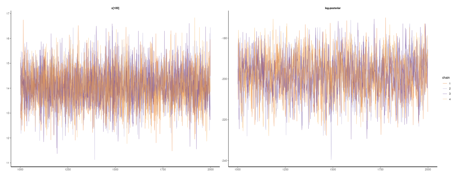
We select two of them, namely state and log posterior probability density at time point 100 and depict them. The trace plot’s horizontal and vertical axes show the number of iterations in the Markov chain and value of the sample, respectively. As mentioned in the beginning of this chapter, the insufficient mixing of multiple Markov chains in a trace plot indicates that some concern remains in the convergence of the chain.
stan_mcmc_out <- rstan::extract(fit_stan, pars = "x")

> dim(stan_mcmc_out$x)
[1] 4000  200
Next, we apply rstan’s function extract() for the object fit_stan to extract only the required sampling result and assign the result to the stan_mcmc_out. Checking the stan_mcmc_out, we see that it is a list whose element $x stores the sampling result. The element $x is a matrix whose rows and columns indicate the iteration number and time, respectively.
Next, we compare this result of smoothing using MCMC with that obtained by Kalman smoothing assuming all the known parameters. While the smoothing result using Stan is a sample from the joint posterior distribution, result obtained using Kalman smoothing is a statistic of the marginal posterior distribution. Thus, we must obtain the required statistics by marginalizing the sample of the joint posterior distribution for the comparison (via colMeans()). The marginalization of a sample from the joint posterior distribution is not difficult: we can achieve the marginalization at a particular time point \(t'\) by considering only the sample at time point \(t'\) while ignoring samples at other time points.
s_mcmc <- colMeans(stan_mcmc_out$x)
s_mcmc_quant <- apply(
  stan_mcmc_out$x,
  2,
  FUN = quantile,
  probs = c(0.025, 0.975)
)

dim(s_mcmc_quant)

dat <- dat |>
  mutate(
    s_mcmc = s_mcmc,
    lower = s_mcmc_quant[1, ],
    upper = s_mcmc_quant[2, ]
  )

dat |>
  autoplot(y, aes(color = "y")) +
  geom_line(
    aes(y = s, color = "s")
  ) +
  geom_line(
    aes(y = s_mcmc, color = "mcmc"),
    linetype = "dashed"
  ) +
  scale_color_manual(
    name = "",
    breaks = c("y", "s", "mcmc"),
    values = c(
      "y" = "lightgray",
      "s" = "blue",
      "mcmc" = "black"
    )
  ) +
  geom_ribbon(
    aes(
      ymax = upper,
      ymin = lower
    ),
    fill = "gray",
    alpha = 0.5
  ) +
  xlab("") +
  theme_tq()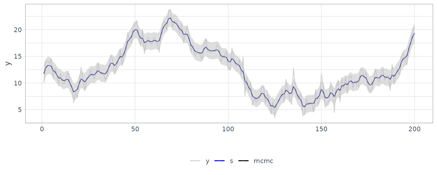
As shown in the above plot, we see that the two results are almost identical. The graph lines overlap and cannot be distinguished from each other. Through the above simple example, we have confirmed that the Stan can accurately estimate the linear Gaussian state-space model.
Example: Estimation in General State-Space Model
We now consider a general state-space model as a linear Gaussian state-space model with unknown parameters treated as random variables. While this section assumes that the parameters of the prior distribution for the state are known as in the previous section, we suppose a situation wherein the variances of the state noise and observation noise are unknown and estimated jointly with the state. The estimation target in this example is now a joint posterior distribution \(p(\textbf{x}_{0:T}, \boldsymbol{\theta} \mid y_{1:T})\), and we obtain samples from that distribution.
// model10-2.stan
// Model: specification
// (local-level model with unknown parameters)

data{
  int<lower=1>   t_max;    // Time series length
  vector[t_max]   y;       // Observations

  real           m0;       // Mean of prior distribution
  cov_matrix[1]  C0;       // Variance of prior distribution
}

parameters{
  real           x0;       // State [0]
  vector[t_max]   x;       // State [1:t_max]

  cov_matrix[1]   W;       // Variance of state noise
  cov_matrix[1]   V;       // Variance of observation noise
}

model{
  //// Likelihood part
  // Observation equation
  for (t in 1:t_max){
    y[t] ~ normal(x[t], sqrt(V[1, 1]));
  }

  //// Prior part
  // Prior distribution for state
  x0 ~ normal(m0, sqrt(C0[1, 1]));

  // State equation
  x[1] ~ normal(x0, sqrt(W[1, 1]));
  for (t in 2:t_max){
    x[t] ~ normal(x[t-1], sqrt(W[1, 1]));
  }
}
We recognize that the variance W of the state noise and variance V of the observation noise are moved from the data block to the parameters block.
Since the distribution of interest in this example is a joint posterior distribution \(p(\textbf{x}_{0:T}, \boldsymbol{\theta} \mid y_{1:T})\), we can specifically transform it according to Bayes’ theorem as follows:
\[\begin{aligned} p(\textbf{x}_{0:T}, \boldsymbol{\theta} | y_{1:T}) &= \frac{p(\textbf{x}_{0:T}, \boldsymbol{\theta}, y_{1:T})}{p(y_{1:T})}\\ &\propto p(\textbf{x}_{0:T}, \boldsymbol{\theta}, y_{1:T})\\ &= p(y_{1:T}|\textbf{x}_{0:T}, \boldsymbol{\theta})p(\textbf{x}_{0:T}, \boldsymbol{\theta})\\ &= \text{likelihood part}\times \text{prior distribution part} \end{aligned}\]We can further show that:
\[\begin{aligned} p(\textbf{x}_{0:T} | y_{1:T}) &= p(\textbf{x}_{0}|\boldsymbol{\theta})\prod_{t=1}^{T}p(y_{t}|\textbf{x}_{t}, \boldsymbol{\theta})p(\textbf{x}_{t}|\textbf{x}_{t-1}, \boldsymbol{\theta})\\ &= \prod_{t=1}^{T}p(y_{t}|\textbf{x}_{t}, \boldsymbol{\theta})\prod_{t=1}^{T}p(\textbf{x}_{t}|\textbf{x}_{t-1}, \boldsymbol{\theta})p(\textbf{x}_{0})p(\boldsymbol{\theta})\\ &= \prod_{t=1}^{T}\text{likelihood part}\prod_{t=1}^{T}\text{prior distribution part} \end{aligned}\]Regarding the \(p(\boldsymbol{\theta})\), we assume that the prior parameters are typically mutually independent unless there is special a priori information. Hence, \(p(\boldsymbol{\theta}) = p(W, V) = p(W)p(V)\) holds. If there is further a priori information on \(p(W), p(V)\), we must reflect that in the code.
The R code:
stan_mod_out <- stan_model(file = "model10-2.stan")

# Smoothing: execution (sampling)
fit_stan <- sampling(
  object = stan_mod_out,
  data = list(
    t_max = t_max,
    y = dat$y,
    m0 = mod$m0,
    C0 = mod$C0
  ),
  pars = c("W", "V", "x"),
  seed = 123
)

> fit_stan
Inference for Stan model: anon_model.
4 chains, each with iter=2000; warmup=1000; thin=1;
post-warmup draws per chain=1000, total post-warmup draws=4000.

          mean se_mean    sd    2.5%     25%     50%     75%   97.5% n_eff Rhat
W[1,1]    0.98    0.01  0.26    0.56    0.79    0.95    1.15    1.58   581 1.00
V[1,1]    2.07    0.01  0.32    1.51    1.85    2.05    2.27    2.74  1570 1.00
x[1]     11.79    0.02  0.97    9.90   11.15   11.80   12.47   13.64  3582 1.00
x[2]     12.82    0.01  0.85   11.13   12.26   12.82   13.42   14.44  4235 1.00
x[3]     13.24    0.01  0.84   11.60   12.67   13.24   13.82   14.89  3925 1.0
...
x[199]   18.63    0.02  0.90   16.82   18.05   18.64   19.24   20.32  2592 1.00
x[200]   19.21    0.02  1.05   17.17   18.51   19.22   19.93   21.25  2722 1.00
lp__   -262.26    0.89 19.58 -299.08 -275.72 -262.59 -249.07 -223.54   479 1.01

Samples were drawn using NUTS(diag_e) at Wed Nov 15 17:26:02 2023.
For each parameter, n_eff is a crude measure of effective sample size,
and Rhat is the potential scale reduction factor on split chains (at
convergence, Rhat=1).
Plotting the traceplot:
tmp_tp <- traceplot(
  fit_stan,
  pars = c("W", "V"),
  alpha = 0.5
)
tmp_tp +
theme(aspect.ratio = 3 / 4) 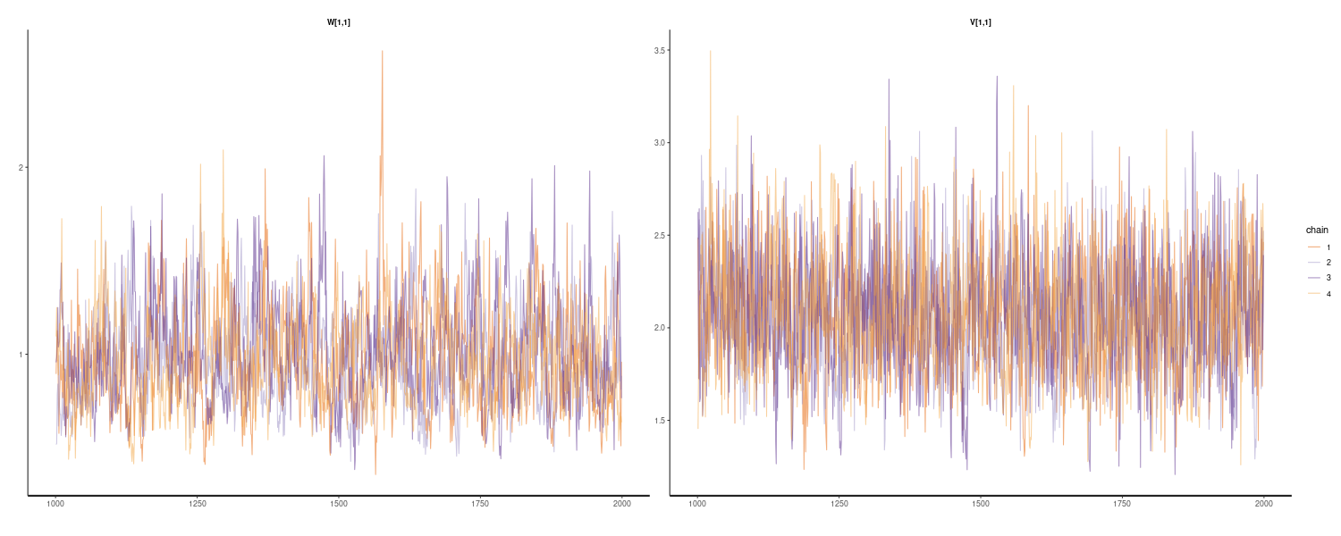
s_mcmc <- colMeans(stan_mcmc_out$x)
s_mcmc_quant <- apply(
  stan_mcmc_out$x,
  2,
  FUN = quantile,
  probs = c(0.025, 0.975)
)

dat <- dat |>
  mutate(
    s_mcmc = s_mcmc,
    lower = s_mcmc_quant[1, ],
    upper = s_mcmc_quant[2, ]
  )
Similar to the previous example, one can’t see the difference between MCMC and Kalman smoothing.
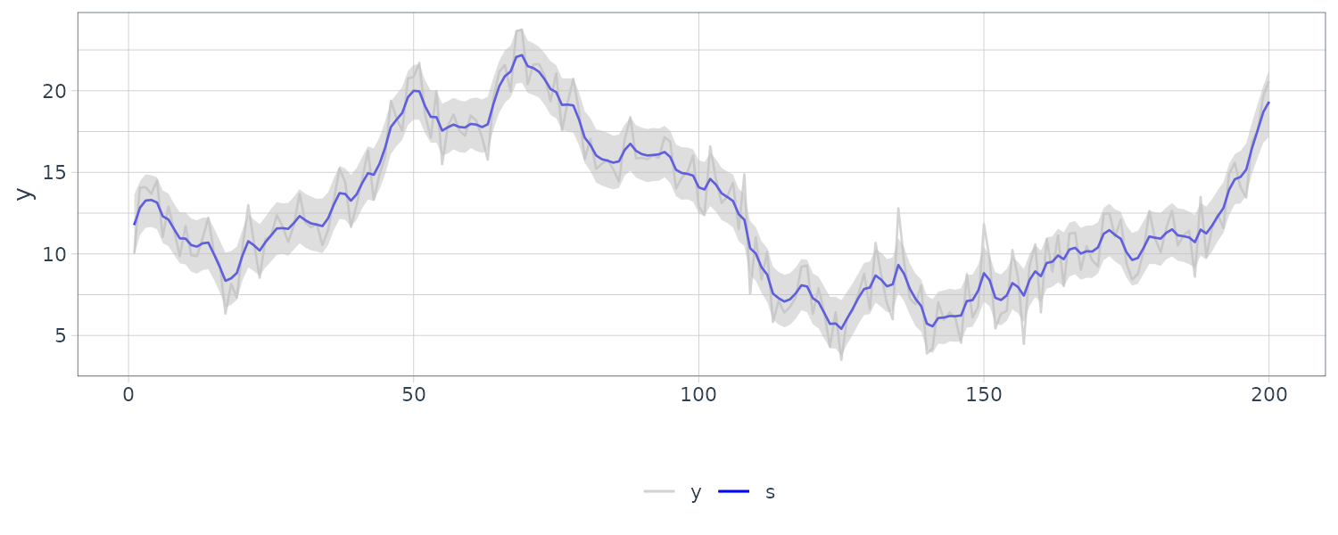
Case in Which the Linear Gaussian State-Space Model is Partially Applicable
In the analysis of the general state-space model, the linear Gaussian state-space model is sometimes, but not always, partially applicable. In such a case, we can use the Kalman filter as a part of the solution. This approach concentrates the finite MCMC ability on the area that cannot be solved using a Kalman filter. In addition, a Kalman filter is an analytical solution and can improve the total estimation accuracy. So whenever possible, we will use this approach.
There are 2 methods that make use of this feature.
First Method
Only parameters are estimated as random variables using MCMC and the estimation result is used in a Kalman filter. In this case, the posterior distribution obtained by MCMC is \(p(\boldsymbol{\theta} \mid y_{1:T})\). Herein, we obtain \(p(\boldsymbol{\theta} \mid y_{1:T}) \propto p(y_{1:T} \mid \boldsymbol{\theta})p(\boldsymbol{\theta})\) from Bayes’ theorem. Since the first term \(p(y_{1:T} \mid \boldsymbol{\theta})\) is the likelihood of the linear Gaussian state-space model, we can use MLE. For the second term \(p(\boldsymbol{\theta})\), if there is no particular prior information, we apply the noninformative prior distribution to it. Finally, we plug the point estimates of \(\boldsymbol{\theta}\) such as the representative value of estimated θ into the Kalman filter.
Stan prepares a function gaussian_dlm_obs() to calculate the likelihood of the linear Gaussian state-space model.
Second Method
We draw a sample from the joint posterior distribution \(p(\textbf{x}_{0:T}, \boldsymbol{\theta} \mid y_{1:T})\) using FFBS. The joint posterior distribution is expanded from Bayes’ theorem as:
\[\begin{aligned} p(\textbf{x}_{0:T}, \boldsymbol{\theta} | y_{1:T}) = p(\textbf{x}_{0:T} | \boldsymbol{\theta}, y_{1:T}) p(\boldsymbol{\theta} | y_{1:T}) \end{aligned}\]For sampling from this distribution, we use the FFBS algorithm. The library dlm provides the function dlmBSample() to execute FFBS. This function calculates Kalman smoothing internally.
Example: Artificial Local-Level Model
While we applied MCMC directly to the same problem for drawing samples of the state previously, we now reproduce the samples of the state using FFBS after parameter estimation. As in the former example, we assume that the mean and variance of the prior distribution for the state are known. Because MCMC here draws only the samples regarding the variances of the state and observation noises, the joint posterior distribution to be estimated becomes:
\[\begin{aligned} p(\boldsymbol{\theta} | y_{1:T}) = p(W , V | y_{1:T}) \end{aligned}\]This code for Stan is as follows:
// model10-3.stan
// Model: specification
// (local-level model with unknown parameters, utilizing Kalman filter)

data{
  int<lower=1>    t_max;   // Time series length
  matrix[1, t_max]    y;   // Observations

  matrix[1, 1]    G;       // State transition matrix
  matrix[1, 1]    F;       // Observation matrix
  vector[1]      m0;       // Mean of prior distribution
  cov_matrix[1]  C0;       // Variance of prior distribution
}

parameters{
  cov_matrix[1]   W;       // Variance of state noise
  cov_matrix[1]   V;       // Variance of observation noise
}

model{
  //// Likelihood part
  // Function calculating likelihood of the linear Gaussian state space model
  y ~ gaussian_dlm_obs(F, G, V, W, m0, C0);

  //// Prior part
  // Prior distribution for W and V:
  // noninformative prior distribution (utilizing the default setting)
}
Next the R code:
set.seed(123)
library(rstan)

stan_mod_out <- stan_model(file = "model10-3.stan")

dim(mod$m0) <- 1

fit_stan <- sampling(
  object = stan_mod_out,
  data = list(
    t_max = t_max,
    y = matrix(dat$y, nrow = 1),
    G = mod$G,
    F = t(mod$F),
    m0 = mod$m0,
    C0 = mod$C0
  ),
  pars = c("W", "V"),
  seed = 123
)

> fit_stan
Inference for Stan model: anon_model.
4 chains, each with iter=2000; warmup=1000; thin=1;
post-warmup draws per chain=1000, total post-warmup draws=4000.

          mean se_mean   sd    2.5%     25%     50%     75%   97.5% n_eff Rhat
W[1,1]    1.00    0.01 0.28    0.57    0.79    0.96    1.15    1.65  1463    1
V[1,1]    2.05    0.01 0.32    1.48    1.83    2.04    2.25    2.73  1782    1
lp__   -235.51    0.02 0.98 -238.13 -235.89 -235.22 -234.80 -234.53  1646    1

Samples were drawn using NUTS(diag_e) at Thu Nov 16 01:12:27 2023.
For each parameter, n_eff is a crude measure of effective sample size,
and Rhat is the potential scale reduction factor on split chains (at
convergence, Rhat=1).
We make mod$m0 a single element vector by providing the explicit dimension. In the argument data of the function sampling(), for accordance with the specification of gaussian_dlm_obs(), we cast the observations y into a one-row matrix and transpose the observation matrix mod$F. In addition, the state x is deleted from the augment pars.
Regarding the sampling results, we see that the effective sample size and Rhat have no particular problem by checking the console display of the fit_stan. The estimated mean values for the variances of the state and observation noises are 1.00 and 2.05, respectively; their true values are 1 and 2, respectively.
Plotting the traceplot:
tmp_tp <- traceplot(
  fit_stan,
  pars = c("W", "V"),
  alpha = 0.5
)
tmp_tp + theme(aspect.ratio = 3 / 4) 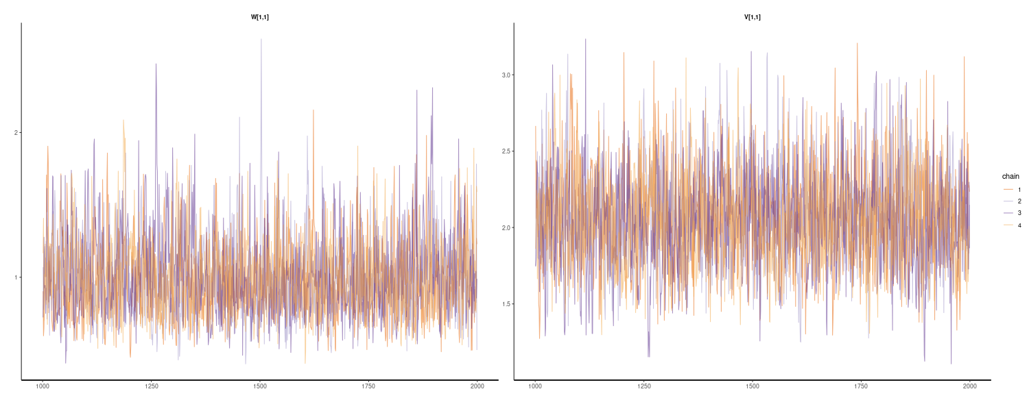
We then reproduce the state sample using FFBS:
set.seed(123)
library(dlm)

stan_mcmc_out <- rstan::extract(
  fit_stan,
  pars = c("W", "V")
)

it_seq <- seq_along(
  stan_mcmc_out$V[, 1, 1]
)

progress_bar <- txtProgressBar(
  min = 1,
  max = max(it_seq),
  style = 3
)

# FFBS main processing: draw of state
x_FFBS <- sapply(
  it_seq,
  function(it) {

    # Display progress bar
    setTxtProgressBar(
      pb = progress_bar,
      value = it
    )

    # Set W and V values in the model
    mod$W[1, 1] <- stan_mcmc_out$W[it, 1, 1]
    mod$V[1, 1] <- stan_mcmc_out$V[it, 1, 1]

    # FFBS execution
    return(
      dlmBSample(
        dlmFilter(
          y = dat$y,
          mod = mod
        )
      )
    )
  }
)

# removal of x0 and transposition
x_FFBS <- t(x_FFBS[-1, ])

s_FFBS <- colMeans(x_FFBS)
s_FFBS_quant <- apply(
  x_FFBS, 2,
  FUN = quantile,
  probs = c(0.025, 0.975)
)

dat <- dat |>
  mutate(
    s_FFBS = s_FFBS,
    lower = s_FFBS_quant[1, ],
    upper = s_FFBS_quant[2, ]
  )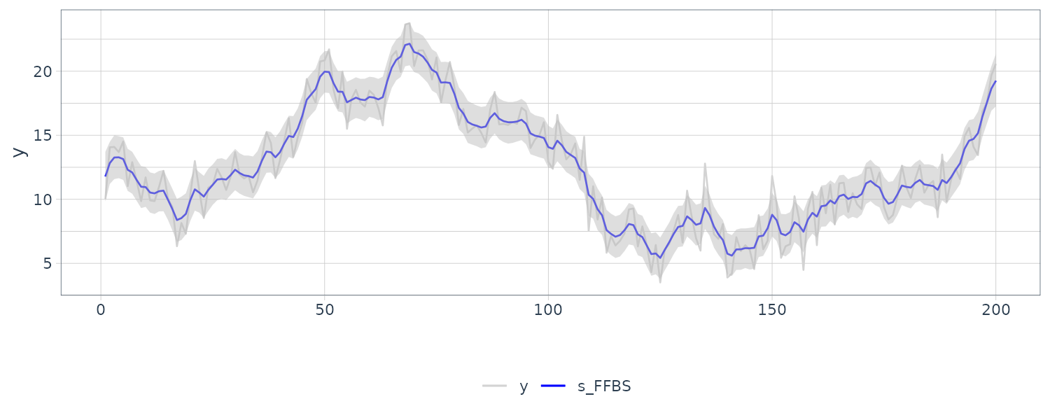
In the processing, realizations of the state and observation noises at a particular MCMC iteration step “it” are set into the model, and state samples are then reproduced using the function dlmBSample(). The argument of the function dlmBSample() is modFilt, which is the output of the function dlmFilter(). Since the state and observation noises in the model vary at every iteration step of MCMC, the function dlmFilter() is executed each time.
Through the above simple example, we have confirmed a method for improving estimation accuracy when the linear Gaussian state-space model is partially applicable.
Example: Monthly Totals of Car Drivers in the UK Killed or Injured
We introduce here an analysis example of monthly totals of car drivers in the UK killed or injured. While various models can be applied to the data, we analyze them with a local-level model + seasonal model (time-domain approach). This model has more states than the local-level model. Recall that the local-level model + seasonal model (time-domain approach) is a linear Gaussian state-space model; when we estimate the state and parameters jointly based on this model, the linear Gaussian state-space model is partially applicable. Thus, we can improve the estimation accuracy and stability with the previously mentioned method using a Kalman filter as parts.
First, we preliminarily examine the data, specify parameters using the maximum likelihood estimation, and apply Kalman smoothing to the data. This code is as follows:
set.seed(123)
library(dlm)

dat <- UKDriverDeaths |>
  as_tsibble() |>
  mutate(
    y = log(UKDriverDeaths)
  )

t_max <- nrow(dat)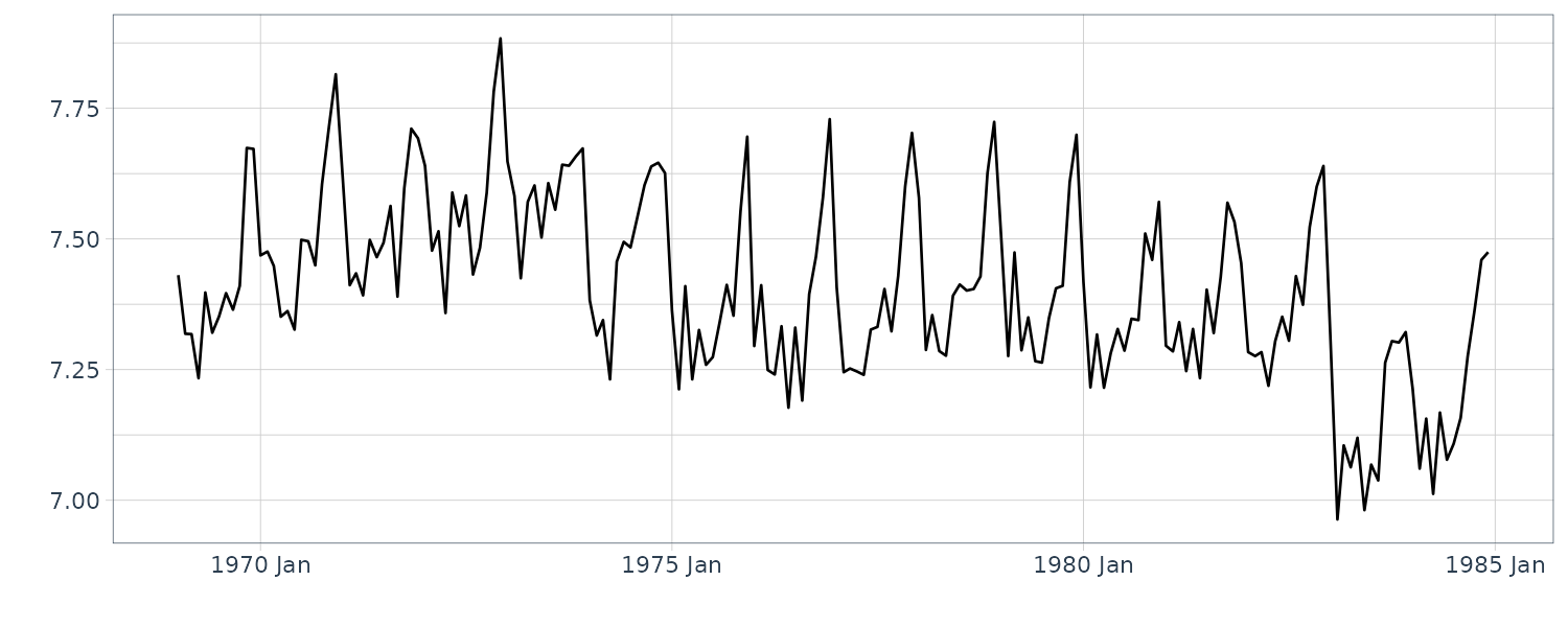
mod <- dlmModPoly(order = 1) +
  dlmModSeas(frequency = 12)

# User-defined function to define and build a model
build_dlm_UKD <- function(par) {
  mod$W[1, 1] <- exp(par[1])
  mod$W[2, 2] <- exp(par[2])
  mod$V[1, 1] <- exp(par[3])

  return(mod)
}

# Maximum likelihood estimation of parameters
fit_dlm_UKD <- dlmMLE(
  y = dat$y,
  parm = rep(0, times = 3),
  build = build_dlm_UKD
)

> fit_dlm_UKD
$par
[1]  -6.963678 -22.419819  -5.651036

$value
[1] -257.4357

$counts
function gradient
      45       45

$convergence
[1] 0

$message
[1] "CONVERGENCE: REL_REDUCTION_OF_F <= FACTR*EPSMCH"


# Model setting and its confirmation
mod <- build_dlm_UKD(fit_dlm_UKD$par)

> cat(diag(mod$W)[1:2], mod$V, "\n")
0.0009456123 1.833144e-10 0.003513874

# Smoothing processing
dlmSmoothed_obj <- dlmSmooth(
  y = dat$y,
  mod = mod
)

# Mean of the smoothing distribution
dat <- dat |>
  mutate(
    mu = dropFirst(dlmSmoothed_obj$s[, 1]),
    gamma = dropFirst(dlmSmoothed_obj$s[, 2])
  )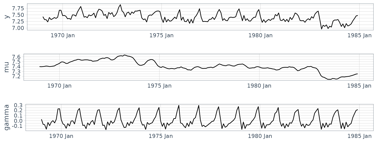
We can recognize the whole level up and down and the distorted annual cycle. We apply dlm functions dlmModPoly() and dlmModSeas() to this data for setting the local-level model + seasonal model (time-domain approach). We use the default setting of these functions; therefore, the mean vector and covariance matrix in the prior distribution of the state are set to \(\textbf{0}\) and \(10^{7}\textbf{I}\), respectively.
The variances of the state noises for the level and seasonal components and the variance of the observation noise are 0.0009456339, 1.841854e-10, and 0.003513928, respectively. These values are not necessarily correct answers because of real data analysis but can be used as a guide.
Subsequently, we draw samples from a joint posterior distribution using Stan. First, we explain the direct means of sampling the state and parameters jointly using MCMC.
This code for Stan is as follows:
// model10-4.stan
// Model: specification
// (local-level model + seasonal model (time-domain approach))

data{
  int<lower=1>    t_max;            // Time series length
  vector[t_max]       y;            // Observations

  vector[12]         m0;            // Mean vector of prior distribution
  cov_matrix[12]     C0;            // Covariance matrix of prior distribution
}

parameters{
  real              x0_mu;          // State (level component) [0]
  vector[11]        x0_gamma;       // State (seasonal component) [0]
  vector[t_max]      x_mu;          // State (level component) [1:t_max]
  vector[t_max]      x_gamma;       // State (seasonal component) [1:t_max]

  real<lower=0>      W_mu;          // Variance of state noise (level component)
  real<lower=0>      W_gamma;       // Variance of state noise (seasonal component)
  cov_matrix[1]      V;             // Covariance matrix of observation noise
}

model{
  //// Likelihood part
  // Observation equation
  for (t in 1:t_max){
    y[t] ~ normal(x_mu[t] + x_gamma[t], sqrt(V[1, 1]));
  }

  //// Prior part
  // Prior distribution for state (level component)
  x0_mu ~ normal(m0[1], sqrt(C0[1, 1]));

  // State equation (level component)
  x_mu[1] ~ normal(x0_mu, sqrt(W_mu));

  for(t in 2:t_max){
    x_mu[t] ~ normal(x_mu[t-1], sqrt(W_mu));
  }

  // Prior distribution for state (seasonal component)
  for (p in 1:11){
    x0_gamma[p] ~ normal(m0[p+1], sqrt(C0[(p+1), (p+1)]));
  }

  // State equation (seasonal component)
  x_gamma[1] ~ normal(-sum(x0_gamma[1:11]), sqrt(W_gamma));

  for(t in 2:11){
    x_gamma[t] ~ normal(-sum(x0_gamma[t:11]) - sum(x_gamma[1:(t-1)]), sqrt(W_gamma));
  }

  for(t in 12:t_max){
    x_gamma[t] ~ normal(-sum(x_gamma[(t-11):(t-1)]), sqrt(W_gamma));
  }

  // Prior distribution for W and V: noninformative prior distribution
  //(utilizing the default setting)
}set.seed(123)
library(rstan)
stan_mod_out <- stan_model(file = "model10-4.stan")
# Smoothing: execution (sampling)
fit_stan <- sampling(
object = stan_mod_out,
data = list(
t_max = t_max,
y = dat$y,
m0 = mod$m0,
C0 = mod$C0
),
pars = c("W_mu", "W_gamma", "V"),
seed = 123
)
# Confirmation of the results
> fit_stan
Inference for Stan model: anon_model.
4 chains, each with iter=2000; warmup=1000; thin=1;
post-warmup draws per chain=1000, total post-warmup draws=4000.
mean se_mean sd 2.5% 25% 50% 75% 97.5% n_eff Rhat
W_mu 0.00 0.00 0.00 0.00 0.00 0.00 0.00 0.00 182 1.01
W_gamma 0.00 0.00 0.00 0.00 0.00 0.00 0.00 0.00 27 1.15
V[1,1] 0.00 0.00 0.00 0.00 0.00 0.00 0.00 0.00 327 1.02
lp__ 1870.29 24.43 89.23 1703.51 1805.36 1867.22 1936.47 2043.55 13 1.24
Samples were drawn using NUTS(diag_e) at Thu Nov 16 03:29:41 2023.
For each parameter, n_eff is a crude measure of effective sample size,
and Rhat is the potential scale reduction factor on split chains (at
convergence, Rhat=1).The traceplot:
tmp_tp <- traceplot(
  fit_stan,
  pars = c("W_mu", "W_gamma", "V"),
  alpha = 0.5
)
tmp_tp + theme(aspect.ratio = 3 / 4)
We see that deterioration of the convergence is detected while executing sampling() and warnings are issued. From the result fit_stan, we also confirm that both effective sample size and Rhat worsen for the variance of the state noise regarding the seasonal component and the log posterior probability. We see from the traceplot that the mixing of estimation results is not good for the variances of state noises (especially regarding the seasonal component).
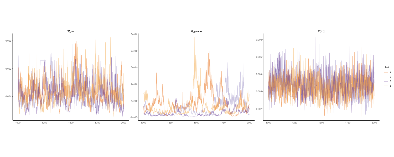
Next, we explain how to sample only parameters using MCMC and then reproduce the state samples using FFBS. This code for Stan is as follows:
// model10-5.stan
// Model: specification
// (local-level model + seasonal model (time-domain approach),
// utilizing Kalman filter)

data{
  int<lower=1>    t_max;           // Time series length
  matrix[1, t_max]    y;           // Observations

  matrix[12, 12]      G;           // State transition matrix
  matrix[12,  1]      F;           // Observation matrix
  vector[12]         m0;           // Mean vector of prior distribution
  cov_matrix[12]     C0;           // Covariance matrix of prior distribution
}

parameters{
  real<lower=0>       W_mu;        // Variance of state noise (level component)
  real<lower=0>       W_gamma;     // Variance of state noise (seasonal component)
  cov_matrix[1]       V;           // Covariance matrix of observation noise
}

transformed parameters{
    matrix[12, 12]    W;           // Covariance matrix of state noise

    // In Stan matrices, the column-major access is effective
    for (k in 1:12){
      for (j in 1:12){
        if (j == 1 && k == 1){
          W[j, k] = W_mu;
        } else if (j == 2 && k == 2){
          W[j, k] = W_gamma;
        } else{
          W[j, k] = 0;
        }
      }
    }
}

model{
  //// Likelihood part
  // Function calculating likelihood of the linear Gaussian state space model
  y ~ gaussian_dlm_obs(F, G, V, W, m0, C0);

  //// Prior part
  // Prior distribution for W and V: noninformative prior distribution
  //(utilizing the default setting)
}
The parameters block declares the parameters to be estimated. In the subsequent transformed parameters block, we can redefine useful parameters by using constants and parameters declared in the data and parameters blocks, respectively. Here, we build a covariance matrix for the state noise. The last model block uses the function gaussian_dlm_obs(). For the prior distribution of the state at time point 0, we use the values stored in mod, that is, mean \(\textbf{0}\) and covariance \(10^{7}\textbf{I}\). We omit any description of the prior distribution for parameters; hence, the default noninformative prior distribution is applied to them.
The R code for executing:
set.seed(123)
library(rstan)

# Model: generation and compilation
stan_mod_out <- stan_model(file = "model10-5.stan")

# Smoothing: execution (sampling)
fit_stan <- sampling(
  object = stan_mod_out,
  data = list(
    t_max = t_max,
    y = matrix(y, nrow = 1),
    G = mod$G,
    F = t(mod$F),
    m0 = mod$m0,
    C0 = mod$C0
  ),
  pars = c("W_mu", "W_gamma", "V"),
  seed = 123
)

# Confirmation of the results
> fit_stan
Inference for Stan model: anon_model.
4 chains, each with iter=2000; warmup=1000; thin=1;
post-warmup draws per chain=1000, total post-warmup draws=4000.

          mean se_mean  sd   2.5%    25%    50%   75%  97.5% n_eff Rhat
W_mu      0.00    0.00 0.0   0.00   0.00   0.00   0.0   0.00  2237    1
W_gamma   0.00    0.00 0.0   0.00   0.00   0.00   0.0   0.00  3729    1
V[1,1]    0.00    0.00 0.0   0.00   0.00   0.00   0.0   0.00  2221    1
lp__    233.22    0.03 1.3 229.87 232.64 233.55 234.2 234.72  1555    1

Samples were drawn using NUTS(diag_e) at Fri Nov 17 02:41:01 2023.
For each parameter, n_eff is a crude measure of effective sample size,
and Rhat is the potential scale reduction factor on split chains (at
convergence, Rhat=1).

tmp_tp <- traceplot(
  fit_stan,
  pars = c("W_mu", "W_gamma", "V"),
  alpha = 0.5
)
tmp_tp + theme(aspect.ratio = 3 / 4)

> cat(
  summary(fit_stan)$summary["W_mu", "mean"],
  summary(fit_stan)$summary["W_gamma", "mean"],
  summary(fit_stan)$summary["V[1,1]", "mean"], "\n"
)
0.001122374 5.059639e-05 0.003354113 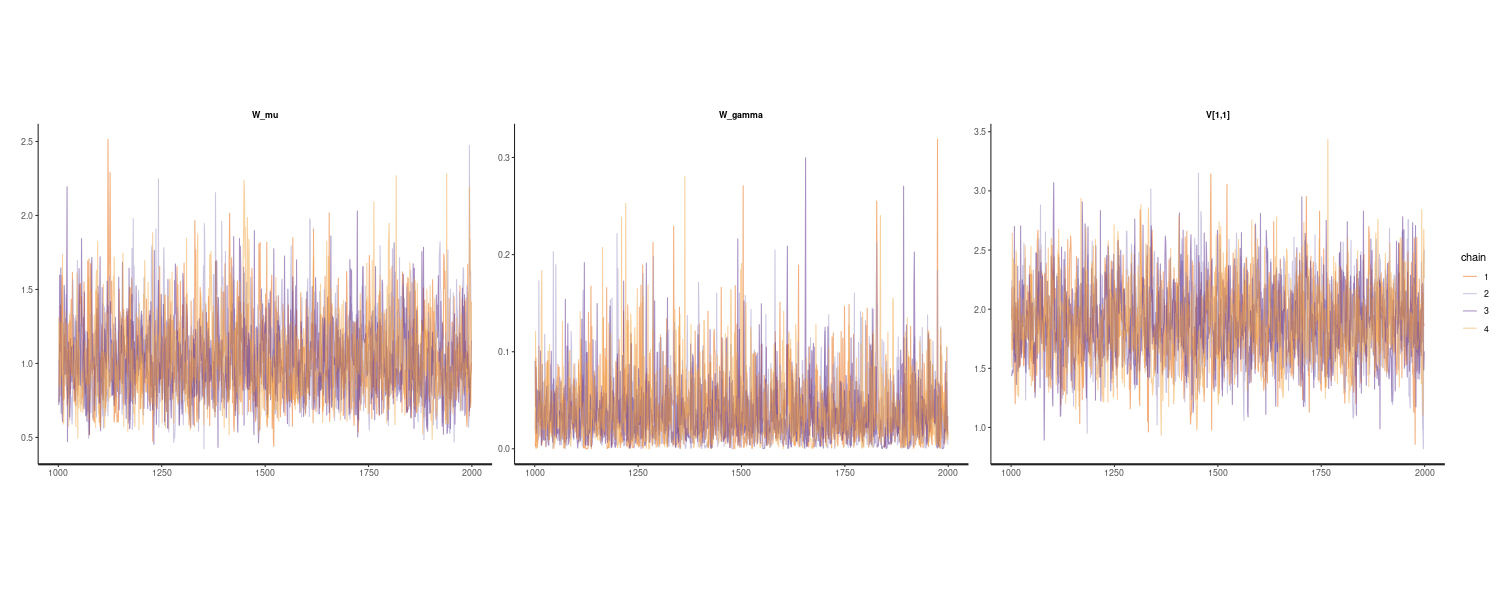
From the result fit_stan, we confirm that both the effective sample size and Rhat are improved. We see in the traceplot that the mixing of estimation results is improved especially for the variance of the state noise regarding the seasonal component. For the parameter estimation result (mean of the marginal distribution), the variances of the state noises for the level & seasonal components and the variance of the observation noise are 0.001134877, 5.002168e-05 and 0.003340325, respectively. While the variance of the state noise for the seasonal component is greater than 1.841854e-10 of the maximum likelihood estimates, we obtain other values close to the maximum likelihood estimates.
Last, we reproduce the state sample using FFBS and compare its statistics to those obtained using Kalman smoothing with parameters specified by maximum likelihood estimation. This code is as follows:
set.seed(123)
library(dlm)

# Extract necessary sampling results
stan_mcmc_out <- rstan::extract(
  fit_stan,
  pars = c("W_mu", "W_gamma", "V")
)

# FFBS preprocessing:
# setting of MCMC iteration step and progress bar
it_seq <- seq_along(stan_mcmc_out$V[, 1, 1])
progress_bar <- txtProgressBar(
  min = 1,
  max = max(it_seq),
  style = 3
)

# FFBS main processing: draw of state
x_FFBS <- lapply(
  it_seq,
  function(it) {
    # Display progress bar
    setTxtProgressBar(pb = progress_bar, value = it)

    # Set W and V values in the model
    mod$W[1, 1] <- stan_mcmc_out$W_mu[it]
    mod$W[2, 2] <- stan_mcmc_out$W_gamma[it]
    mod$V[1, 1] <- stan_mcmc_out$V[it, 1, 1]

    # FFBS execution
    return(
      dlmBSample(
        dlmFilter(
          y = dat$y, mod = mod
        )
      )
    )
  }
)

# FFBS post-processing:
# removal of x0 and transposition
x_mu_FFBS <- t(
  sapply(
    x_FFBS,
    function(x) {
      x[-1, 1]
    }
  )
)
x_gamma_FFBS <- t(
  sapply(
    x_FFBS,
    function(x) {
      x[-1, 2]
    }
  )
)

# Calculate the mean while marginalizing
dat <- dat |>
  mutate(
    mu_FFBS = colMeans(x_mu_FFBS),
    gamma_FFBS = colMeans(x_gamma_FFBS)
  )

plot_grid(
  dat |>
    autoplot(y, alpha = 0.5) +
    geom_line(aes(y = mu), col = "blue") +
    geom_line(aes(y = mu_FFBS), col = "red") +
    xlab("") +
    theme_tq(),
  dat |>
    autoplot(gamma) +
    geom_line(aes(y = gamma_FFBS), col = "red") +
    xlab("") +
    theme_tq(),
  ncol = 1
)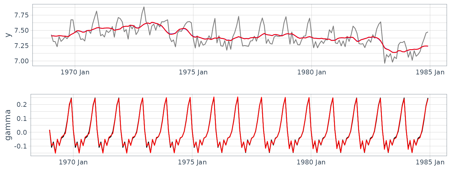
We see that the two sets of results are almost identical. The graph lines overlap and cannot be distinguished from each other. Confirming carefully, we can see a slight deviation for the graph regarding the mean of the seasonal component. This result appears to be influenced by the fact that the variance of the state noise regarding the seasonal component is estimated to be greater than the maximum likelihood estimates. However, we cannot see a big difference overall for the mean of the marginal smoothing distribution.
Through the above example, we have confirmed that the stability of the estimation for a complex model can be improved by using a Kalman filter as parts when the linear Gaussian state-space model is partially applicable.
Example of Applied Analysis in General State-Space Model
Consideration of Structural Change
This chapter discusses the flow data of the Nile again as time series data with structural change. This chapter aims to properly consider the rapid decrease in the flow in 1899, which is associated with the construction of the Aswan (Low) Dam. As a study step, we first review the case with the known change point and then extend the idea to the case wherein the change point is unknown.
Incidentally, although this chapter examines a method that appropriately considers the structural change included in time series data, such change point detection is also known as a type of anomaly detection. Regarding time series data with a known change point, we have already introduced a method using the regression model.
This section now discusses an alternative approach that considers time-varying state noise variance. By considering the parameters as time-varying, we can improve the ability to follow the structural change. Thus far, while we have considered that the parameters are basically time-invariant, we henceforth treat the time-varying case as well. Then, note that we refer to the term time-varying or time-invariant parameter as simply time-varying or time-invariant, respectively.
Furthermore, we extend the concept of the time-varying parameter for the case wherein the change point is unknown. We apply a fat-tailed distribution to the state noise specifically. Such a distribution makes it easy for the state noise to take a very large value. Since the state noise is the tolerance for the temporal change of the state, a situation wherein its value occasionally becomes large can adequately explain the fact that the state value changes suddenly and significantly.
As a solution in the following discussion, while a Kalman filter is applied to the “known” change point, MCMC and a particle filter are applied to the “unknown” change point. In addition, for the estimation type, we use fixed-interval smoothing to compare the results under identical conditions.
Approach Using a Kalman Filter (Known Change Point)
Recall this local-level model is defined by:
\[\begin{aligned} x_{t} &= x_{t-1} + w_{t}\\ y_{t} &= x_{t-1} + v_{t} \end{aligned}\] \[\begin{aligned} w_{t} &\sim N(0, W)\\ v_{t} &\sim N(0, V) \end{aligned}\]We now modify the definition of the state noise in the local-level model. Specifically, we suppose that the variance of the state noise increases “only” in 1899 to ensure that we can include the influence of rapid change in that year to the model appropriately. While such an approach makes the variance of the state noise time-varying, we treat the change point as not unknown but known. Hence, the model still follows the linear Gaussian state-space model. Such a local-level model is defined as follows:
\[\begin{aligned} x_{t} &= x_{t-1} + w_{t}\\ y_{t} &= x_{t-1} + v_{t} \end{aligned}\] \[\begin{aligned} w_{t} &\sim N(0, W_{t})\\ v_{t} &\sim N(0, V) \end{aligned}\]Specifically, \(W_{t}\) is set as \(W_{\text{other than 1899}} = W\) and \(W_{\text{1899}} = \lambda^{2}W\). While W is time-invariant and is common throughout all the years, the factor \(\lambda^{2}\) exists only for 1899. Incidentally, we refer to a Kalman filter for the linear Gaussian state-space models with such time-varying parameters as a time-varying Kalman filter.
The code for executing the time-varying Kalman filter:
set.seed(123)
library(dlm)

# Flow data of the Nile

dat <- as_tsibble(Nile)
dat <- dat |>
  rename(
    y = value
  )
t_max <- nrow(dat)

build_dlm <- function(par) {
  mod <- dlmModPoly(
    order = 1,
    dV = exp(par[1])
  )

  # Variance of state noise refers to the first column of X
  mod$JW <- matrix(
    1,
    nrow = 1,
    ncol = 1
  )

  # Store the variance of state noise in the first column of X
  mod$X <- matrix(
    exp(par[2]),
    nrow = t_max,
    ncol = 1
  )

  # Allow increase of state noise only in 1899
  j <- which(dat$index == 1899)
  mod$X[j, 1] <- mod$X[j, 1] * exp(par[3])

  return(mod)
}

# Maximum likelihood estimation of parameters
fit_dlm <- dlmMLE(
  y = dat$y,
  parm = rep(0, 3),
  build = build_dlm
)
modtv <- build_dlm(fit_dlm$par)
> as.vector(modtv$X)
[1] 6.709260e-02 6.709260e-02 6.709260e-02 6.709260e-02 6.709260e-02
... 6.035191e+04 6.709260e-02 6.709260e-02 6.709260e-02 6.709260e-02
[34] 6.709260e-02 6.709260e-02 6.709260e-02 6.709260e-02 6.709260e-02
...

> modtv$V
          [,1]
[1,] 16301.65

# Kalman filtering
dlmFiltered_obj <- dlmFilter(
  y = dat$y,
  mod = modtv
)

# Mean of the smoothing distribution
dat <- dat |>
  mutate(
    stv = dropFirst(dlmFiltered_obj$m),
    sdev = sqrt(
      dropFirst(
        as.numeric(
          dlmSvd2var(
            dlmFiltered_obj$U.C,
            dlmFiltered_obj$D.C
          )
        )
      )
    ),
    lower = stv + qnorm(0.025, sd = sdev),
    upper = stv + qnorm(0.975, sd = sdev)
  )

# Kalman smoothing
dlmSmoothed_obj <- dlmSmooth(
  y = dat$y,
  mod = modtv
)

# Mean of the smoothing distribution
dat <- dat |>
  mutate(
    stv = dropFirst(dlmSmoothed_obj$s)
  )

dat |>
  autoplot(y, alpha = 0.5) +
  geom_line(aes(y = stv), col = "blue") +
  xlab("") +
  theme_tq()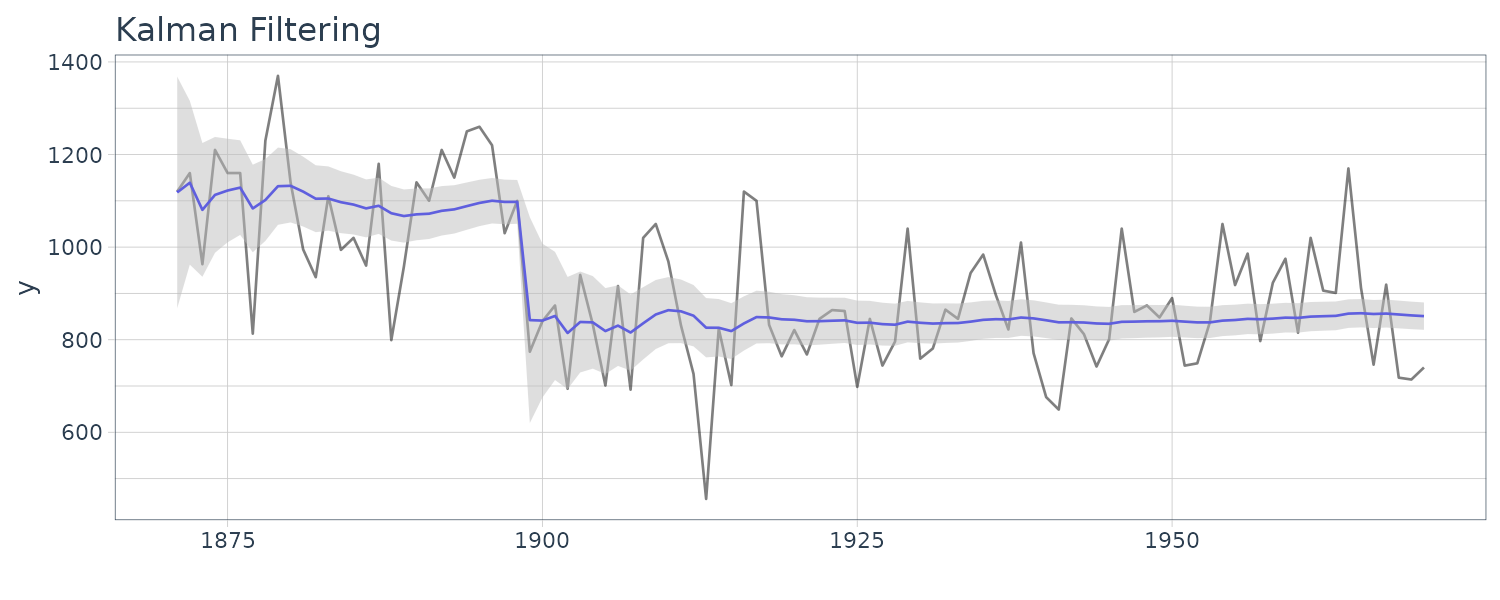
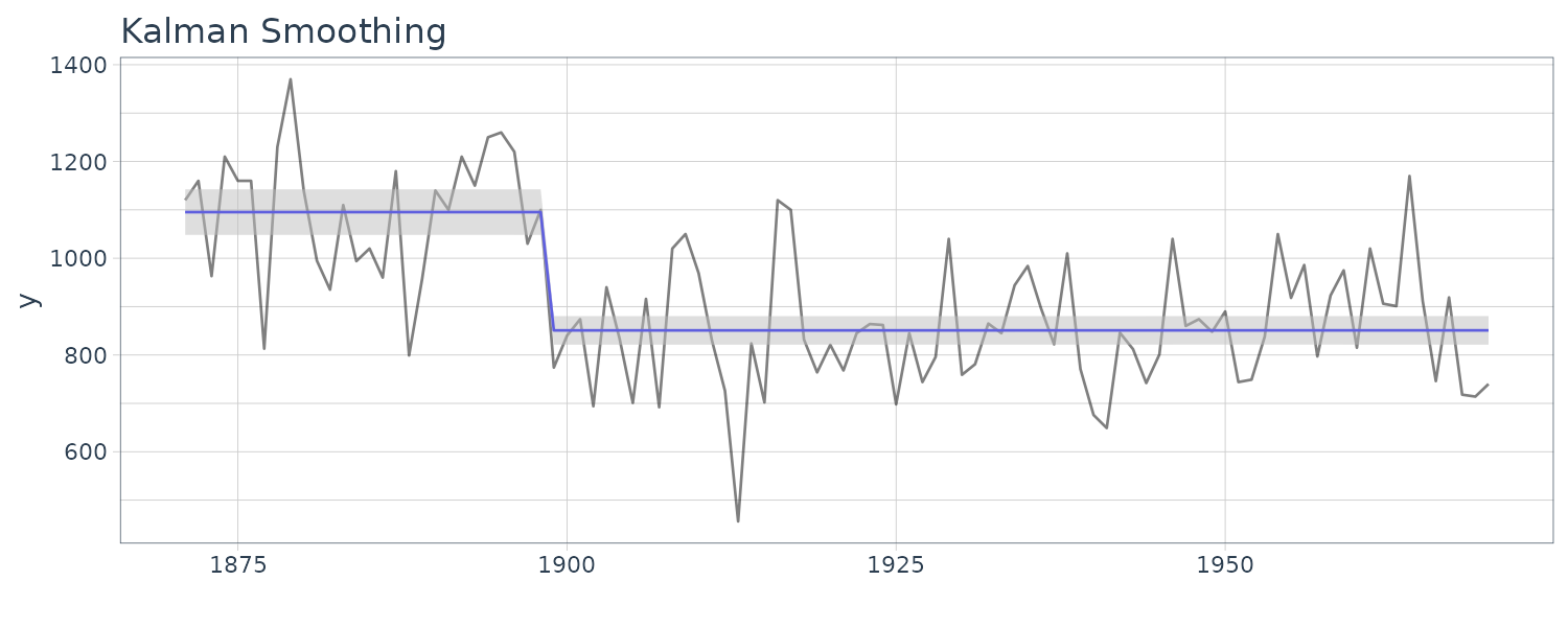
We prepare the user-defined function build_dlm() to create a time-varying model. Inside this function, we first create the model template mod using function dlmModPoly(). We then set the mod$JW to one (a 1 × 1 matrix) considering the time-varying variance of the state noise.
Regarding the time-varying variance, the values are stored in the first column of mod$X. Thus, we set the unique time-invariant base value to all of them and then overwrite the specific value to ensure that it can have a positive factor only in 1899.
Next, the maximum likelihood method specifies the parameters using this modelbuilding function build_dlm(). The variances \(W_{t}\) of the state noise are specified as 6.709260e-02 except in 1899; the variance in 1899 is 6.035191e+04, and the variance V of the observation noise is specified as 16301.65. The above figure shows a plot for the mean of the smoothing distribution obtained from the Kalman smoother with the above-specified parameters.
Furthermore, we see that the estimated level is almost constant before and after 1899. While this is not necessarily the correct answer because of the real data analysis, this chapter considers this result as a guideline for rapid change in 1899.
Approach Using MCMC (Unknown Change Point)
Use of a Horseshoe Distribution in the General State-Space Mode
In the previous section, we specified a time-varying model based on the prior information regarding a historical fact. However, such information is not always available. To properly consider a rarely occurring structural change even without prior information, we try to apply a distribution other than the normal distribution to the state noise.
If we can assume the degree of “rare” to some extent, it might be better to use mixtures of Gaussians. On the contrary, it is typical to use a fat-tailed distribution in a circumstance wherein we cannot clearly assume such a degree. While the t-distribution and Cauchy distribution (t-distribution with one degree of freedom) are often used as a fat-tailed distribution, the horseshoe distribution has recently been proposed. This distribution can enhance the thickness of the tail and concentration around the mode. The horseshoe distribution is defined through a scale mixture of the normal distribution as follows:
\[\begin{aligned} \text{Horseshoe Distribution}(\text{center} = 0, \text{scale} = \sigma) &= N(0, \lambda_{t}^{2}\sigma^{2}) \end{aligned}\] \[\begin{aligned} \lambda_{t} &\sim \mathcal{C}^{+}(\text{center} = 0, \text{scale} = 1) \end{aligned}\]Where \(\mathcal{C}^{+}\) is the Cauchy distribution whose support is limited positive and is referred to as a half-Cauchy distribution. The above equation implies that the normal distribution becomes a horseshoe distribution by considering the time-varying factor \(\lambda_{t}\), which follows the half-Cauchy distribution, to the scale (standard deviation) of the normal distribution. As can be seen from the equation, the time-varying factor is usually less than 1 but is sometimes large; hence, while the horseshoe distribution almost yields a value smaller than \(\sigma\) , it sometimes yields a large value.
The horseshoe distribution is suitable for expressing the sparsity because of the thickness of the tail and the high concentration around the mode. While the Laplace (double exponential) distribution is also used for expressing sparsity, the horseshoe distribution can enhance further the concentration around the mode.
A further feature of the horseshoe distribution is its computational advantage. Since this distribution is expressed as a scale mixture of the normal distribution from the definition, we can use the linear Gaussian state-space model conditionally. Herein, the scale factor \(\lambda_{t}\) is time-varying. This implies that the solution requires a time-varying Kalman filter.
Based on the abovementioned attractive features, we apply the horseshoe distribution to the state noise. In this case, the local-level model \(w_{t}\) is defined as follows:
\[\begin{aligned} w_{t} &\sim \text{Horseshoe Distribution}(\text{center} = 0, \text{scale} = \sqrt{W}) \end{aligned}\]Thus, while \(w_{t}\) usually takes a value smaller than W, it sometimes takes a large value.
We now examine an example wherein the state noise follows the horseshoe distribution. When we use a horseshoe distribution, the conditional linear Gaussian state-space model requires a time-varying Kalman filter for the solution.
The function gaussian_dlm_obs() in Stan 2.19.2 does not yet support the time-varying linear Gaussian state-space model. Regarding this point, while future revision is expected, Dr. Jeffrey B. Arnold, who contributed to the implementation of gaussian_dlm_obs(), has implemented a time-varying Kalman filter as a user-defined function. We can download the source code from https://raw.githubusercontent.com/jrnold/dlm-shrinkage/master/stan/includes/dlm.stan and then decide to use this function in the analysis below.
// model12-1.stan
// Model: specification (local-level model +
// horseshoe distribution with unknown parameters,
// utilizing time-varying Kalman filter)

/*
 * The contents of the forefront function block are borrowed
 * from the following site (partly modified to avoid the latest
 * rstan's warning)
 * https://raw.githubusercontent.com/jrnold/dlm-shrinkage/master
 * /stan/includes/dlm.stan
 */

functions{
  // -*- mode: stan -*-
  // --- BEGIN: dlm ---

  // ...
}

data{
  int<lower = 1>              t_max;  // Time series length
  vector[t_max]                   y;  // Observations
  int                   miss[t_max];  // Indicator for missing values
  real                           m0;  // Mean of prior distribution
  real<lower = 0>                C0;  // Variance of prior distribution
}

parameters{
  // Standard deviation of state noise (time-varying factor)
  vector<lower = 0>[t_max]   lambda;

  // Standard deviation of state noise (time-invariant base)
  real<lower = 0>          W_sqrt;

  // Standard deviation of observation noise (time-invariant)
  real<lower = 0>          V_sqrt;
}

transformed parameters{
  // Variance of state noise (time-varying)
  vector[t_max]                   W;

  // Variance of observation noise (time-varying)
  vector[t_max]                   V;

  // Log-likelihood through all time points
  real                      log_lik;

  // Variance of state noise
  // (different value is set at every time point)
  for (t in 1:t_max) {
    W[t] = pow(lambda[t] * W_sqrt, 2);
  }

  // Variance of observation noise (unique value is set at all time points)
  V = rep_vector(pow(V_sqrt, 2), t_max);

  // The final log-likelihood
  log_lik = sum(dlm_local_level_loglik(t_max, y, miss, V, W, m0, C0));
}

model{
  //// Likelihood part
  target += log_lik;

  //// Prior part
  // Standard deviation of state noise (time-varying factor)
  lambda ~ cauchy(0, 1);

  // Standard deviation of state noise (time-invariant base)
  // and standard deviation of observation noise (time-invariant):
  // noninformative prior distribution
}
At the beginning of the above code, the functions block describes the user-defined functions. In the block, we define various functions, such as a generic function that performs Kalman filtering to time-varying linear Gaussian state-space models and specialized function dlm_local_level_loglik() for time-varying local-level modes.
This example uses the latter specialized function. The arguments of this function are the time series length “t_max”, data “y”, missing observations index “miss”, time-varying variance “V” of the observation noise, time-varying variance “W” of the state noise, mean m0 of the prior distribution, and variance C0 of the prior distribution.
In the following data block, we set t_max, y, miss, m0, and C0. These data types are consistent with the arguments of the function dlm_local_level_loglik().
In the following parameters block, we declare the scale factor lambda for the standard deviation of the state noise, standard deviation W_sqrt (time-invariant base) of the state noise, and standard deviation V_sqrt (time-invariant) of the observation noise.
In the following transformed parameters block, we first transform the parameters declared in the parameters block to ensure that they match the arguments of the function dlm_local_level_loglik(). Specifically, the time-varying variance W of the state noise is set according to Horeshoe distribution, and the time-varying variance V of the observation noise is set to a unique value at all time points. In addition, since the function dlm_local_level_loglik() can obtain the vectors of log-likelihoods for all time points, we sum them to derive the entire log-likelihood log_lik.
In the following model block, we describe the posterior distribution. In the likelihood part, we use the notation “target += log-likelihood”, which directly describes the log-likelihood instead of “observations ~ likelihood”.
In the prior distribution part, we apply the half-Cauchy distribution to the prior distribution for the lambda. We added the condition <lower = 0> at the declaration of lambda, resulting in the range of its sample being limited positive. We omit the description of the prior distributions for the standard deviation (time-invariant base) of the state noise and standard deviation (time-invariant) of the observation noise; hence, the noninformative prior distributions are applied to them.
The R code:
set.seed(123)
library(rstan)

# Model: generation and compilation
stan_mod_out <- stan_model(file = "model12-1.stan")

# Smoothing: execution (sampling)
fit_stan <- sampling(
  object = stan_mod_out,
  data = list(
    t_max = t_max,
    y = dat$y,
    miss = as.integer(is.na(dat$y)),
    m0 = modtv$m0,
    C0 = modtv$C0[1, 1]
  ),
  pars = c("lambda", "W_sqrt", "V_sqrt"),
  seed = 123
)

> print(fit_stan, probs = c(0.025, 0.5, 0.975))
Inference for Stan model: anon_model.
4 chains, each with iter=2000; warmup=1000; thin=1;
post-warmup draws per chain=1000, total post-warmup draws=4000.

               mean se_mean     sd    2.5%     50%   97.5% n_eff Rhat
lambda[1]      4.10    0.46  28.01    0.03    0.97   23.57  3631 1.00
lambda[2]      2.84    0.19  10.49    0.03    0.94   17.93  3089 1.00
lambda[3]      2.69    0.12   6.86    0.04    0.97   16.76  3107 1.00
...
W_sqrt         4.61    0.09   4.15    0.41    3.47   15.05  1960 1.00
V_sqrt       128.11    0.18  10.36  109.28  127.56  149.67  3432 1.00
lp__        -768.15    0.27   9.32 -787.87 -767.50 -751.20  1154 1.01

Samples were drawn using NUTS(diag_e) at Fri Nov 17 18:35:03 2023.
For each parameter, n_eff is a crude measure of effective sample size,
and Rhat is the potential scale reduction factor on split chains (at
convergence, Rhat=1).

tmp_tp <- traceplot(
  fit_stan,
  pars = c("W_sqrt", "V_sqrt"),
  alpha = 0.5
)
tmp_tp + theme(aspect.ratio = 3 / 4)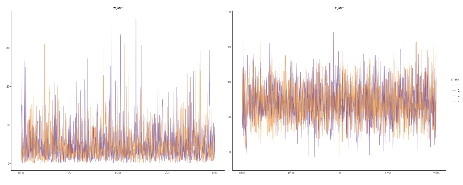
modtv_MCMC <- modtv
modtv_MCMC$X[, 1] <- (
  summary(fit_stan)$summary[1:100, "mean"] *
    summary(fit_stan)$summary["W_sqrt", "mean"]
)^2
modtv_MCMC$V[1, 1] <- (
  summary(fit_stan)$summary["V_sqrt", "mean"]
)^2

> as.vector(modtv_MCMC$X)
[1]    356.86929    171.09844    153.94167    180.24867
...
[100]    225.10864

> modtv_MCMC$V
          [,1]
[1,] 16412.03

# Kalman smoothing
dlmSmoothed_obj <- dlmSmooth(
  y = dat$y,
  mod = modtv_MCMC
)

# Mean of the smoothing distribution
dat <- dat |>
  mutate(
    stv_MCMC = dropFirst(dlmSmoothed_obj$s)
  )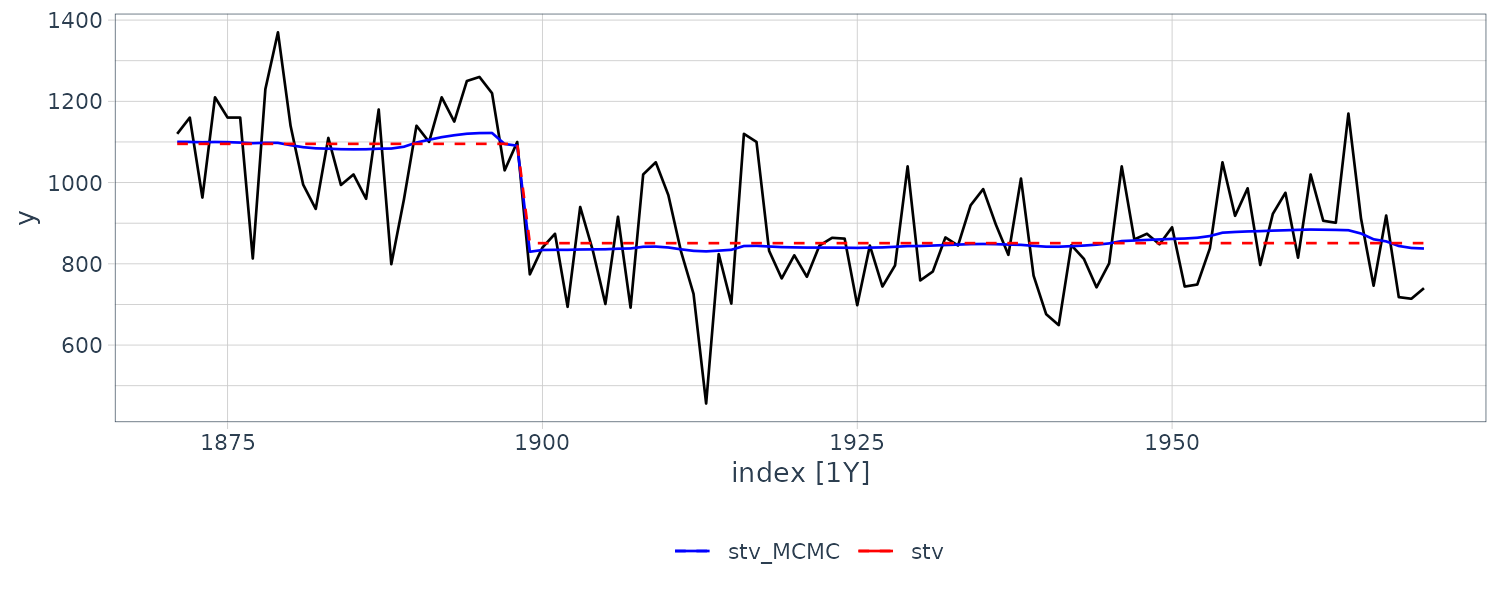
The data type for the argument of the function sampling() conforms to the specification of the function dlm_local_level_loglik(). The argument miss is a vector of all 0s because the data y in this example have no missing observations.
From the result, we can confirm that neither the effective sample size nor Rhat have any particular problem. There is no particular problem shown in the traceplot with their mixing.
Finally, we derive the smoothing distribution of the state using a time-varying Kalman filter. We copy the time-varying model modtv prepared previously to the modtv_MCMC, and then we make necessary corrections to it. Specifically, we substitute the estimated mean values using MCMC into the X and V, which store the time-varying variance of the state noise and time-invariant variance of the observation noise, respectively.
Confirming the contents of the time-varying variance of the state noise, we see that it takes the maximum value of 303593.721 in 1899 (29th-time point) and smaller values at other time points. In addition, the variance of the observation noise takes the value of 16384.74, which is close to the maximum likelihood estimates. In the plot, we see that the level before and after 1899 shows some fluctuation compared with that obtained using time-varying Kalman smoothing.
The model is a simple structure expressing the data characteristics. It is com mon to think of combining simpler structures in defining a model; this is also known as decomposition of time series data. This chapter explicitly considers “level + trend + season” as a starting point since this is widely recognized as a fundamental decomposition of time series data. Additionally, the remainders resulting from subtracting these estimated components from the original time series data are referred to as residuals.
The basic concept of modeling is the same even in the advanced state-space model. A typical model and combinations of them are the basic. In the state-space model, the model corresponding to “level + trend + season” is referred to as the basic structural model or standard seasonal adjustment model.
See Also
References
Hagiwara J. (2021) Time Series Analysis for the State-Space Model with R/Stan
