Time Series Modeling
Read PostIn this post, we will cover Kitagawa G. (2021) Introduction to Time Series Modeling.
Contents:
Datasets
Let us look at the datasets we will be using in this post. All the datasets can be found in the TSSS package.
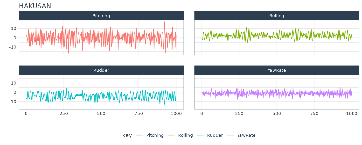
HAKUSAN
A multivariate time series of a ship’s yaw rate, rolling, pitching and rudder angles which were recorded every second while navigating across the Pacific Ocean.
Graphing the YawRate against time:
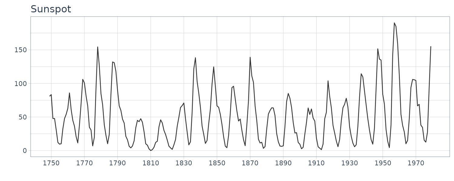
Sunspot
Yearly numbers of sunspots from to 1749 to 1979.
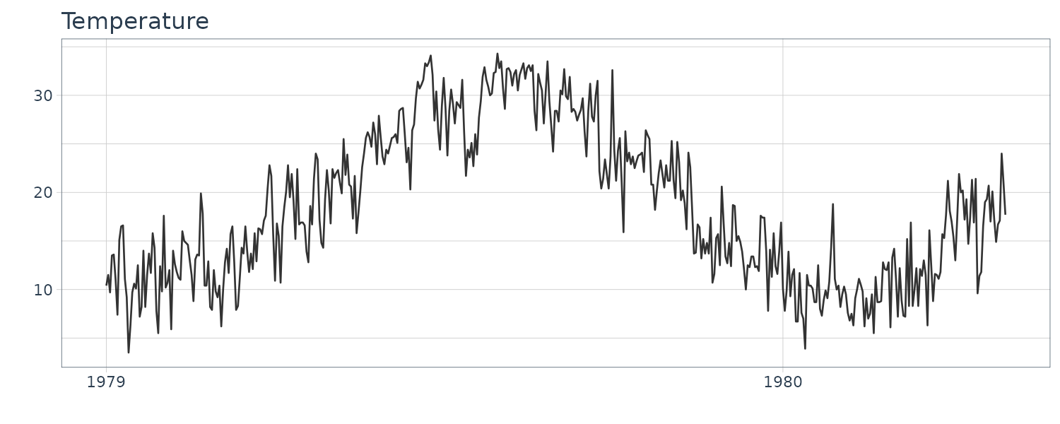
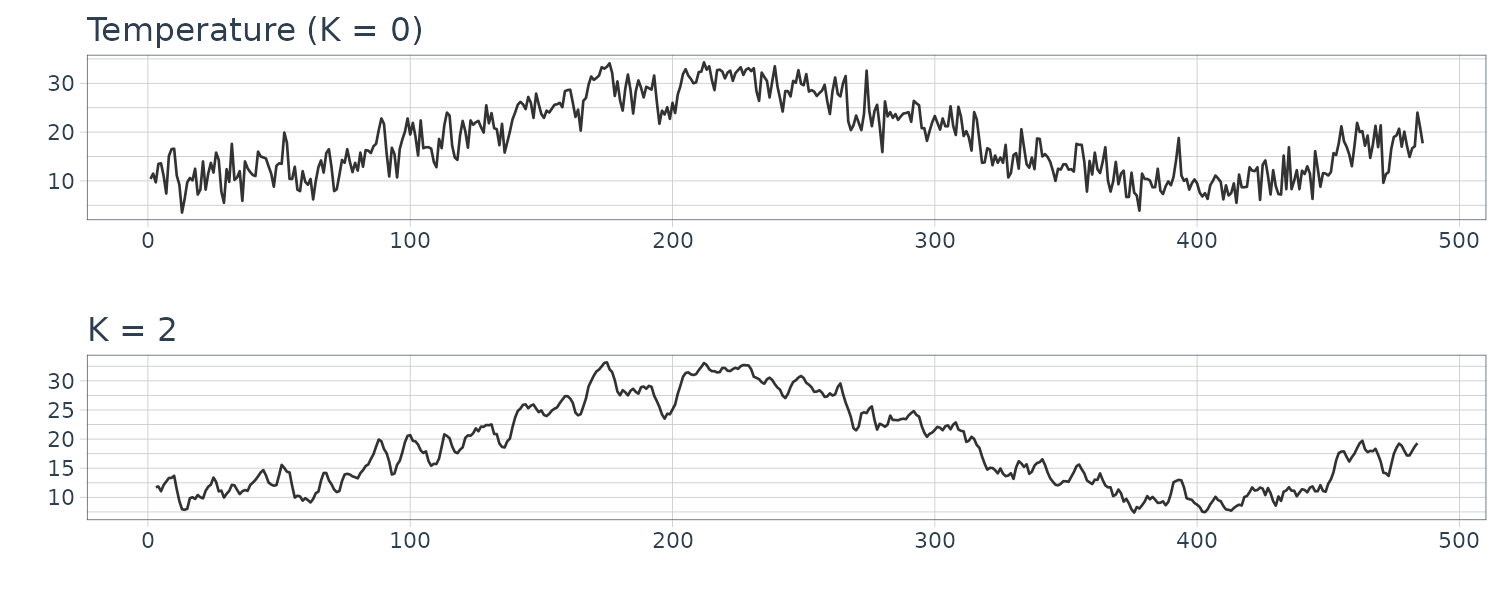
Temperature
The daily maximum temperatures in Tokyo (from 1979-01-01 to 1980-04-30).
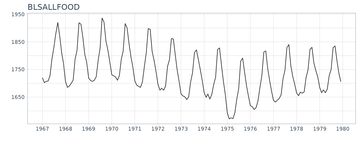
BLSALLFOOD
The monthly time series of the number of workers engaged in food industries in the United States (January 1967 - December 1979).
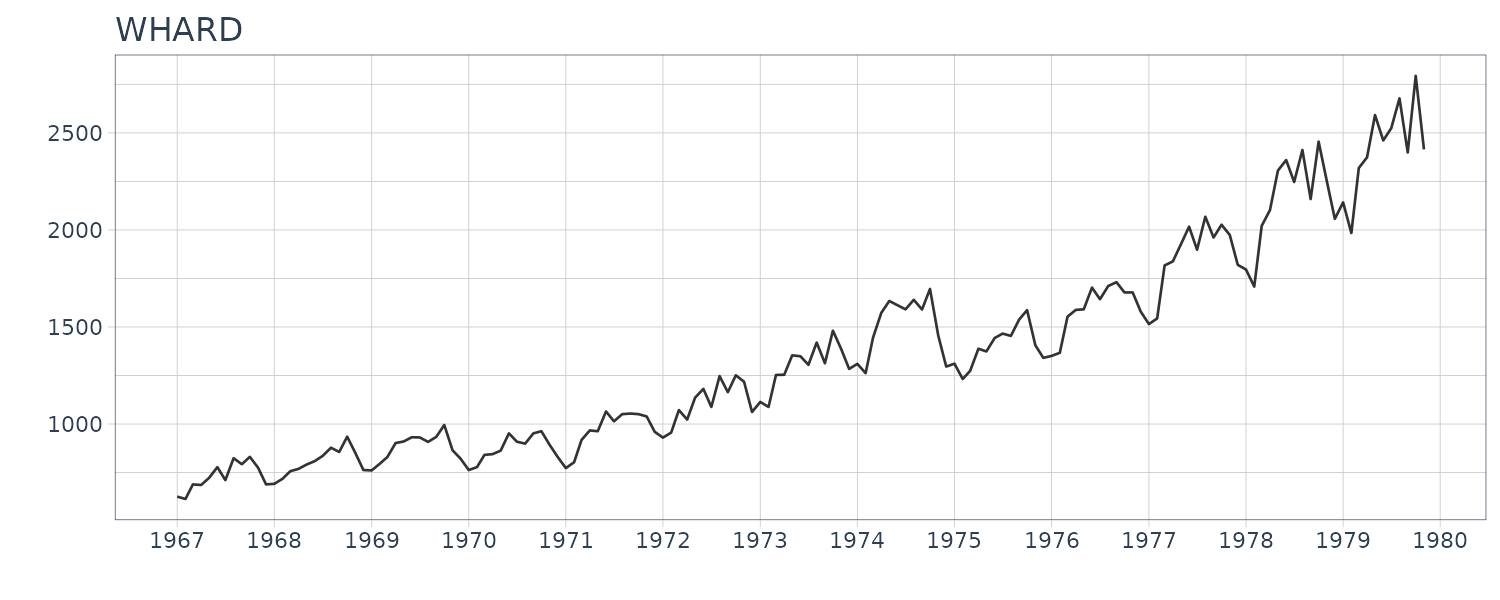
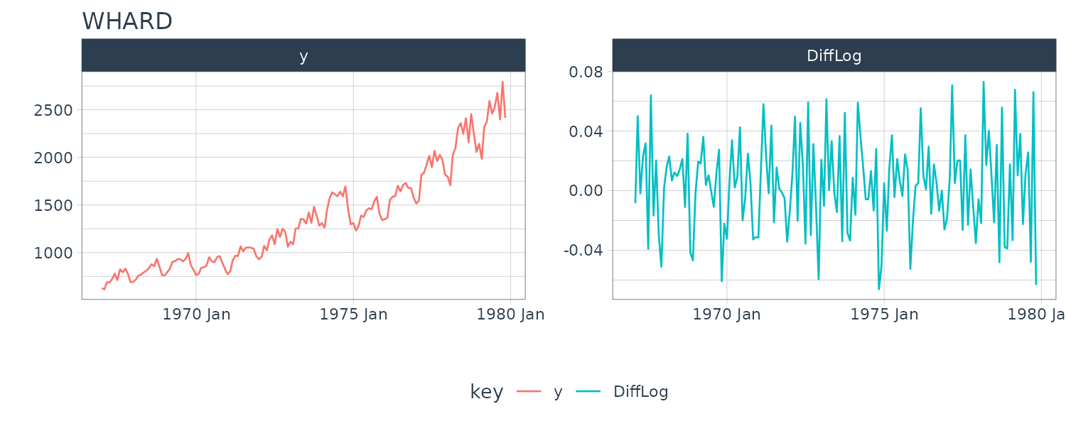
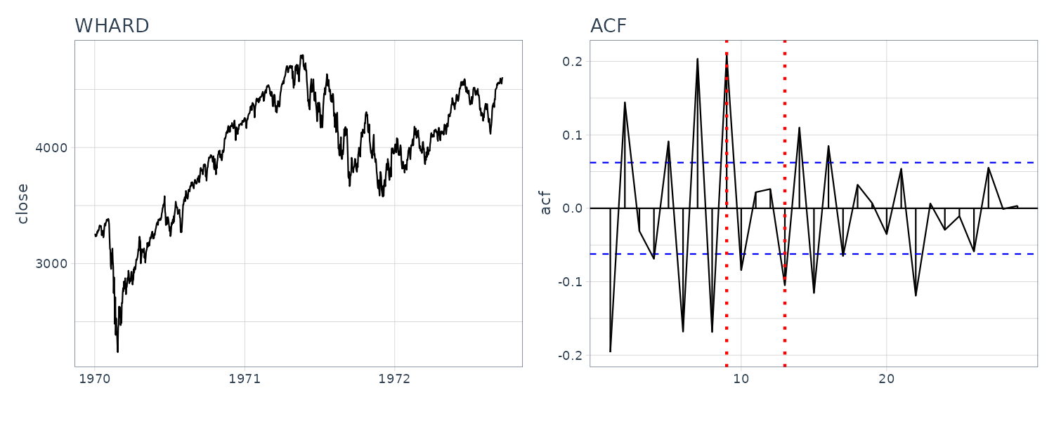
WHARD
The monthly record of wholesale hardware data. (January 1967 - November 1979)
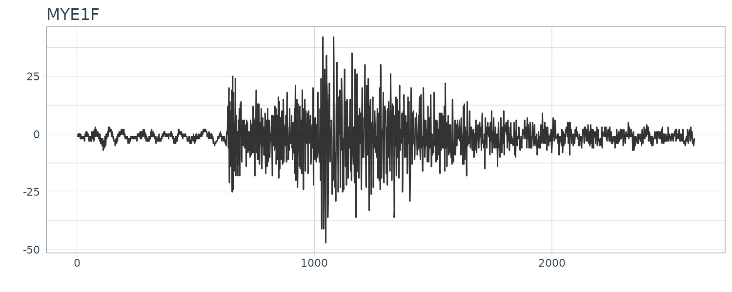
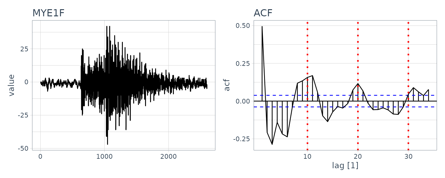
MYE1F
The time series of East-West components of seismic waves, recorded every 0.02 seconds.
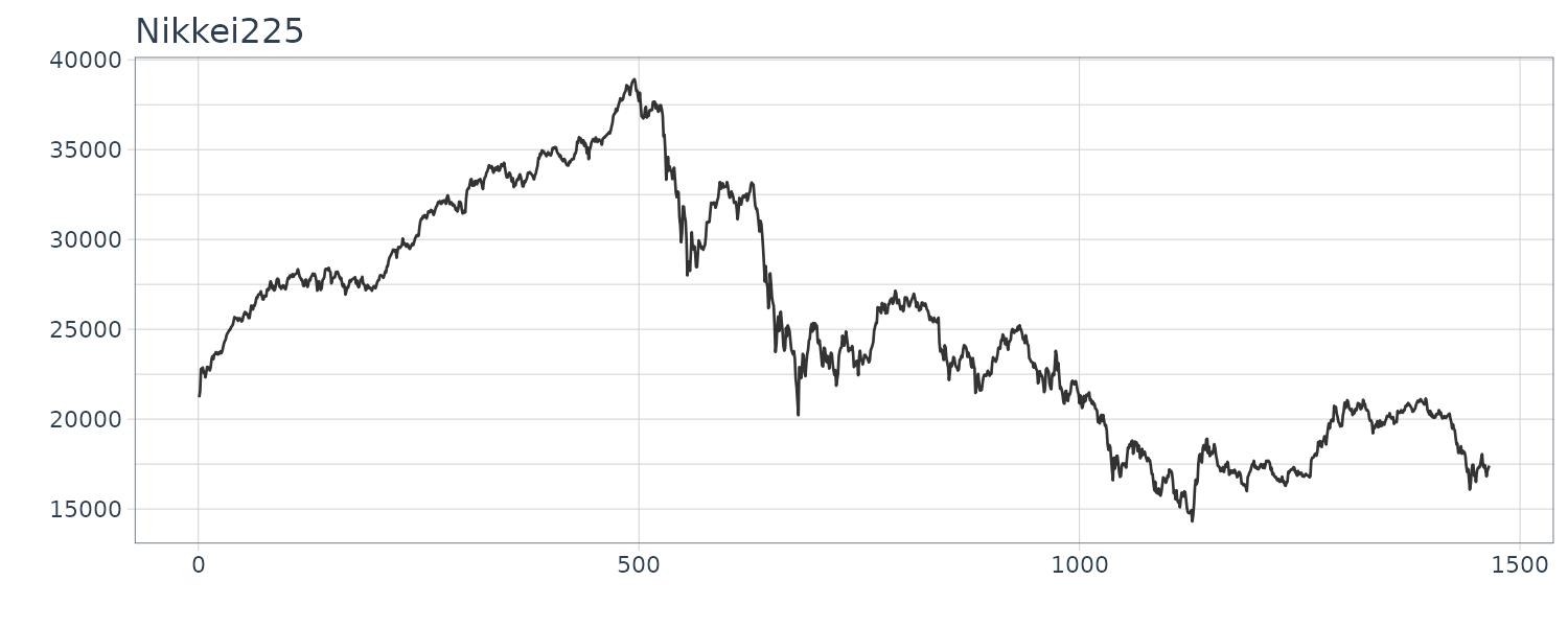
Nikkei225
A daily closing values of the Japanese stock price index, Nikkei225, quoted from January 4, 1988, to December 30, 1993.
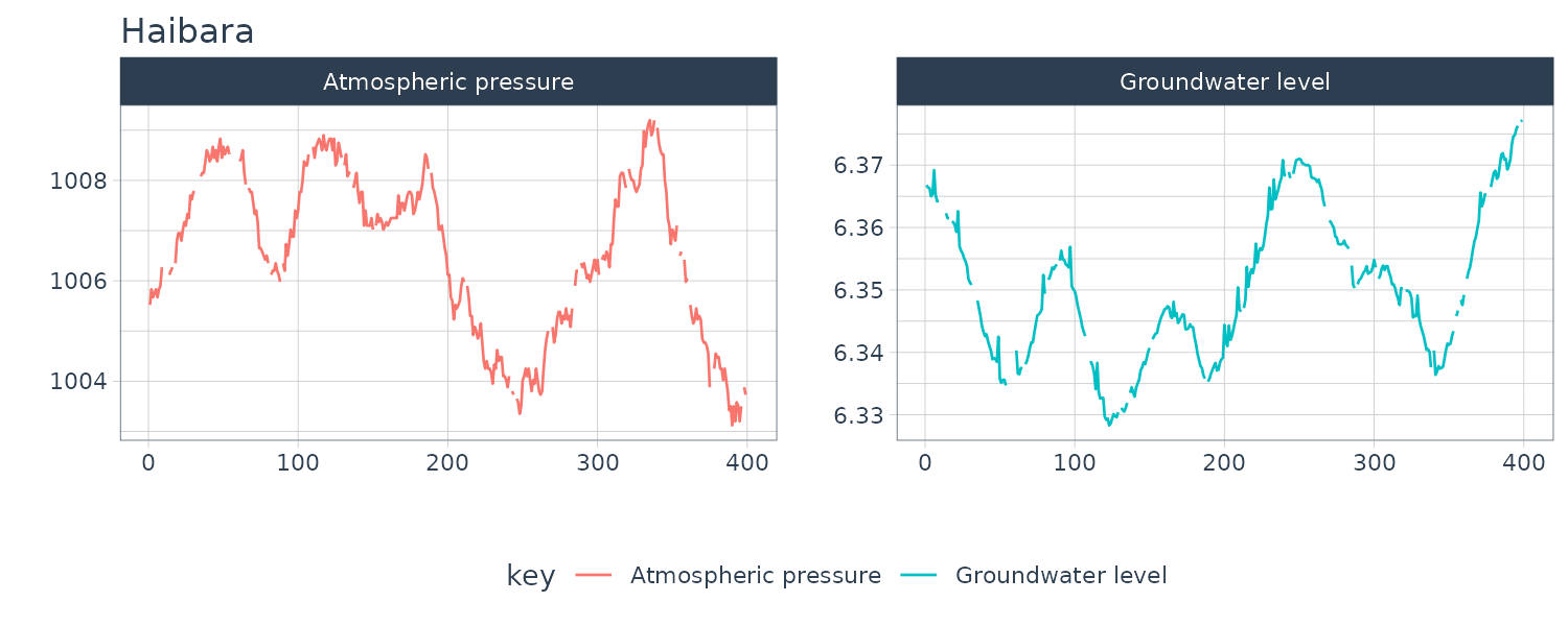
Haibara
A bivariate time series of the groundwater level and the atmospheric pressure that were observed at 10-minuite intervals at the Haibara observatory of the Tokai region, Japan.
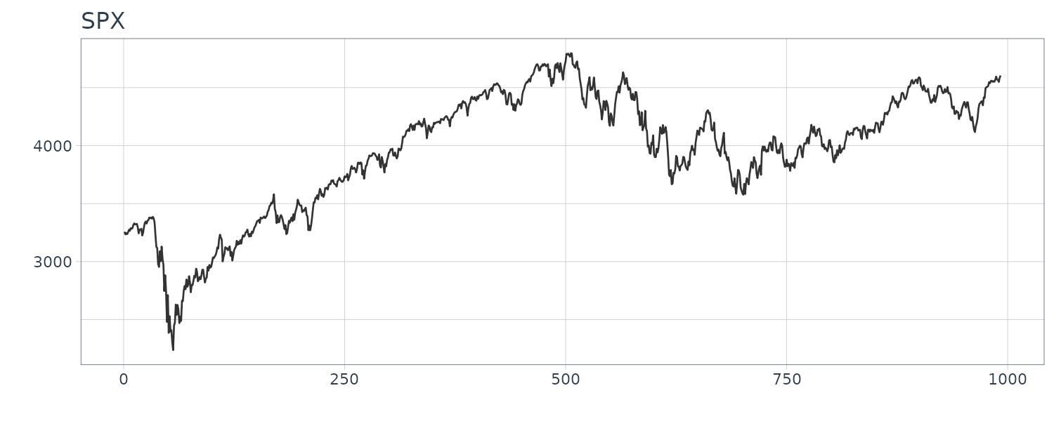
SPX
And finally we add our own SPX index (not from TSSS) dataset which consists of the close price from January 1, 2020, to December 10, 2023.
Transformation of Variables
Log-Transformation
Some types of time series obtained by counting numbers or by measuring a positive-valued process such as the prices of goods and numbers of people. They share the common characteristic that the variance of the series increases as the level of the series increases. For such a situation, by using the log-transformation \(z_{n} = \log y_{n}\), we may obtain a new series whose variance is almost time-invariant and noise distribution is closer to the normal distribution than the original series \(y_{n}\).
For example, we plot the log-transformed of WHARD data. It can be seen that the log-transformed data is actually almost uniform and the trend of the series becomes almost linear:
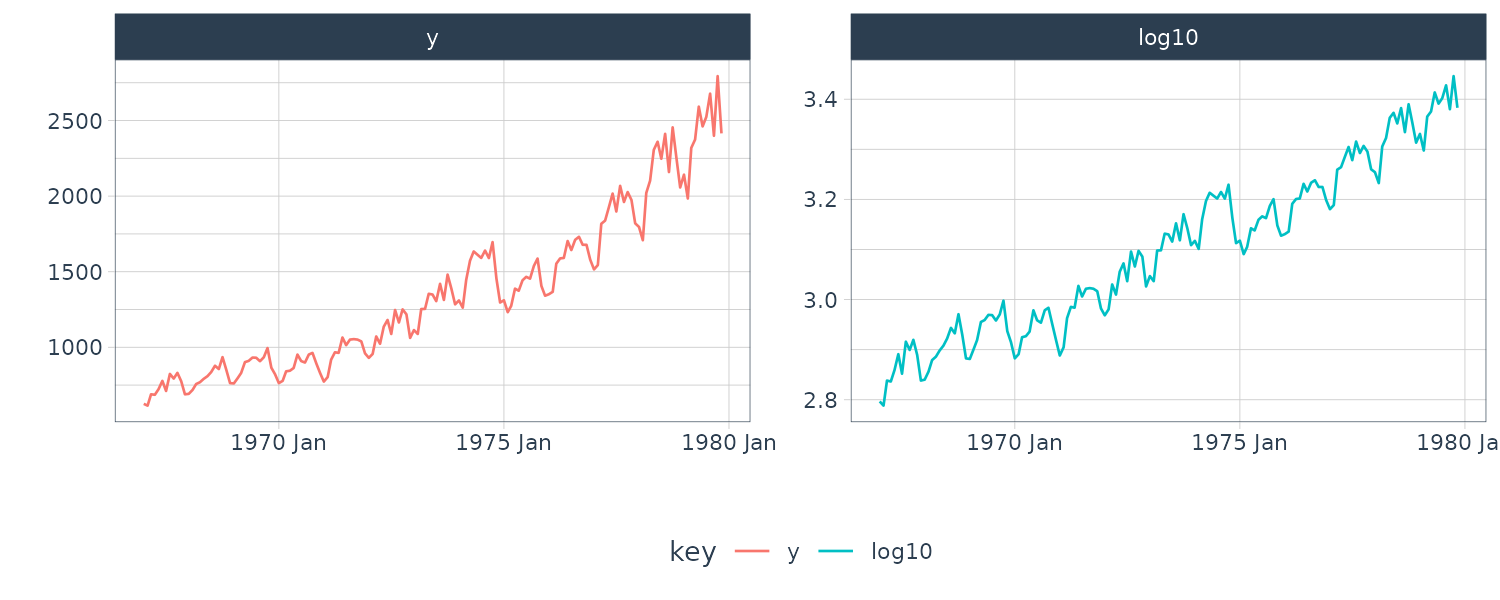
A more general Box-Cox transformation includes the log-transformation as a special case and the automatic determination of its parameter will be considered later.
Differencing
When a time series \(y_{n}\) contains a trend, we often analyze the differenced series \(z_{n}\) defined as:
\[\begin{aligned} z_{n} &= \Delta y_{n}\\ &= y_{n} - y_{n-1} \end{aligned}\]This is motivated by the fact that if \(y_{n}\) is a straight line expressed as \(y_{n} = a + bn\), then the differenced series:
\[\begin{aligned} z_{n} &= \Delta y_{n}\\ &= b \end{aligned}\]And the slope of the straight line can be removed.
For example, taking a difference on the log-transformed WHARD dataset:
Furthermore, if \(y_{n}\) follows the quadratic function \(y_{n} = a + bn + cn^{2}\), the difference of \(z_{n}\) becomes a constant and a and b are removed as follows:
\[\begin{aligned} z_{n} &= \Delta y_{n}\\ &= a + bn + cn^{2} - (a + b(n-1) + c(n-1)^{2})\\ &= b(n - n - 1) + cn^{2} - c(n^{2} - 2n + 1))\\ &= -b + 2cn - c\\ &= c(2n - 1) - b \end{aligned}\] \[\begin{aligned} \Delta z_{n} &= z_{n}- z_{n-1}\\ &= \Delta y_{n} - \Delta y_{n-1}\\ &= c(2n - 1) - b - (c(2(n-1) - 1) - b)\\ &= 2cn - c - (2cn - 2c - c)\\ &= 2cn - 2cn - c + 2c + c\\ &= 2c \end{aligned}\]For economic time series with prominent trend components as shown in, changes in the time series \(y_{n}\) from the previous month (or quarter) or year-over-year changes are often considered:
\[\begin{aligned} z_{n} &= \frac{y_{n}}{y_{n-1}}\\ x_{n} &= \frac{y_{n}}{y_{n-p}} \end{aligned}\]Where \(p\) is the cycle length or the number of observations in one year.
If the time series \(y_{n}\) is represented as the product of the trend \(T_{n}\) and the noise \(w_{n}\) as
\[\begin{aligned} y_{n} &= T_{n}w_{n} \end{aligned}\]Where \(\alpha\) is the growth rate:
\[\begin{aligned} T_{n} &= (1 + \alpha)T_{n-1} \end{aligned}\]Then the change from the previous month can be expressed by:
\[\begin{aligned} z_{n} &= \frac{y_{n}}{y_{n-1}}\\ &= \frac{T_{n}w_{n}}{T_{n-1}w_{n-1}}\\ &= (1 + \alpha)\frac{w_{n}}{w_{n-1}} \end{aligned}\]This means that if the noise can be disregarded, the growth rate \(\alpha\) can be determined by this transformation.
On the other hand, if \(y_{n}\) is represented as the product of a periodic function \(s_{n}\) with the cycle \(p\) and the noise \(w_{n}\):
\[\begin{aligned} y_{n} &= s_{n}w_{n}\\ s_{n} &= s_{n-p} \end{aligned}\]The the year-over-year \(x_{n}\) can be expressed by:
\[\begin{aligned} x_{n} &= \frac{y_{n}}{y_{n-p}}\\ &= \frac{s_{n}w_{n}}{s_{n-p}w_{n-p}}\\ &= \frac{w_{n}}{w_{n-p}} \end{aligned}\]This suggests that the periodic function is removed by this transformation.
Moving Average
For a time series \(y_{n}\), the \((2k + 1)\)-term moving average of \(y_{n}\) is defined by:
\[\begin{aligned} T_{n} &= \frac{1}{2k+1}\sum_{j=-k}^{k}y_{n+j} \end{aligned}\]When the original time series is represented by the sum of the straight line tn and the noise \(w_{n}\) as:
\[\begin{aligned} y_{n} &= t_{n} + w_{n}\\ t_{n} &= a + bn \end{aligned}\]Then:
\[\begin{aligned} T_{n} &= t_{n} + \frac{1}{2k + 1}\sum_{j=-k}^{k}w_{n+j}\\ E[T_{n}] &= t_{n} + \frac{1}{2k + 1}\sum_{j=-k}^{k}E[w_{n+j}]\\ &= t_{n}\\ \textrm{var}(T_{n}) &= \frac{1}{(2k+1)^{2}}\sum_{j=-k}^{k}\textrm{var}(w_{n+j})\\ &= \frac{1}{(2k+1)^{2}}\sum_{j=-k}^{k}E[w_{n+j}^{2}]\\ &= \frac{1}{(2k+1)^{2}}(2k+1)\sigma^{2}\\ &= \frac{\sigma^{2}}{2k+1} \end{aligned}\]This shows that the mean of the moving average \(T_{n}\) is the same as that of \(t_{n}\) and the variance is reduced to \(\frac{1}{2k + 1}\) of the original series \(y_{n}\).
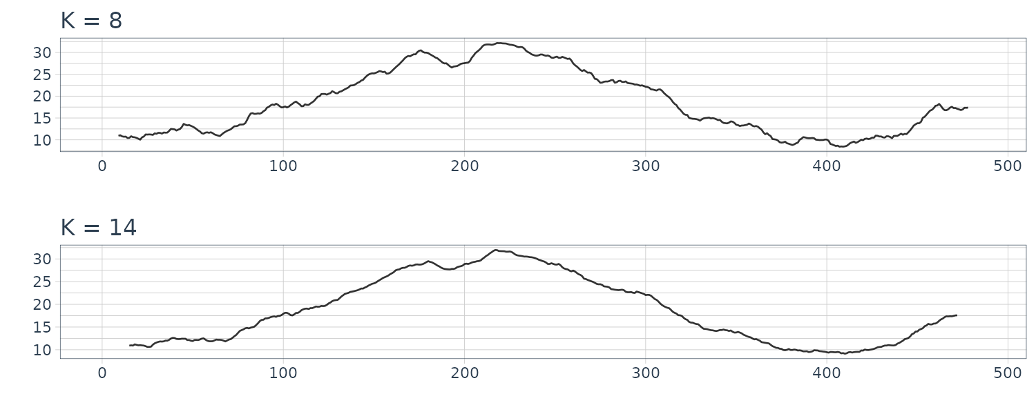
dat <- Temperature |>
  rename(
    y = value
  ) |>
  mutate(
    K2 = stats::filter(
      y,
      sides = 2,
      filter = rep(1 / 5, 5)
    ),
    K8 = stats::filter(
      y,
      sides = 2,
      filter = rep(1 / 17, 17)
    ),
    K14 = stats::filter(
      y,
      sides = 2,
      filter = rep(1 / 29, 29)
    ),
  )
Covariance Function
The autocovariance function is a tool to express the relation between past and present values of time series and the cross-covariance function is to express the relation between two time series.
These covariance functions are used to capture features of time series, to estimate the spectrum and to build time series models.
It is not possible to capture the essential features of time series by the marginal distribution of \(y_{n}\) that is obtained by ignoring the time series structure. Consequently, it is necessary to consider not only the distribution of \(y_{n}\) but also the joint distribution of \(\{y_{n}, y_{n−1}\}\), \(\{y_{n}, y_{n−2}\}\), and in general \(\{y_{n}, y_{n−k}\}\). The properties of these joint distributions can be concisely expressed by the use of covariance and correlation coefficients of \(\{y_{n}, y_{n−k}\}\).
Given a time series \(y_{1}, \cdots, y_{N}\), the expectation of \(y_{n}\) is defined as:
\[\begin{aligned} \mu_{n} &= E[y_{n}] \end{aligned}\]And the covariance at two different times \(y_{n}\) and \(y_{n-k}\) is defined as:
\[\begin{aligned} \text{Cov}(y_{n}, y_{n-k}) &= E[(y_{n} - \mu_{n})(y_{n-k} - \mu_{n-k})] \end{aligned}\]For \(k = 0\), we get the variance:
\[\begin{aligned} \text{Var}(y_{n}) &= E[y_{n} - \mu_{n}]^{2} \end{aligned}\]Stationarity
In this section, we consider the case when the mean, the variance and the covariance do not change over time \(n\).
That is, we assume that for an arbitrary integer \(k\), it holds that:
\[\begin{aligned} E[y_{n}] &= E[y_{n-k}]\\[5pt] \text{Var}(y_{n}) &= \text{Var}(y_{n-k})\\[5pt] \text{Cov}(y_{n}, y_{m}) &= \text{Cov}(y_{n-k, m - k}) \end{aligned}\]The time series is known as covariance stationary or weakly stationary. If the mean and covariance change over time, it is known as nonstationary.
If the data is further Gaussian distributed, the characteristics of the distribution is completely determined by the mean, variance, and covariance.
The features of a time series cannot always be captured completely only by the mean, the variance and the covariance function. In general, it is necessary to examine the joint probability density function of the time series:
\[\begin{aligned} f(y_{i_{1}}, \cdots, y_{i_{N}}) \end{aligned}\]For that purpose, it is sufficient to specify the joint probability density function for arbitrary integers k:
\[\begin{aligned} f(y_{i_{1}}, \cdots, y_{i_{k}}) \end{aligned}\]In particular, when this joint distribution is a k-variate normal distribution, the time series is called a Gaussian time series. The features of a Gaussian time series can be completely captured by the mean vector and the variance covariance matrix.
When the time series is invariant with respect to time, meaning that the distribution does not change with time and the pdf satisfy the following relation:
\[\begin{aligned} f(y_{i_{1}}, \cdots, y_{i_{k}}) &= f(y_{i_{1} - l}, \cdots, y_{i_{k}- l}) \end{aligned}\]The time series is known as strongly stationary. As Gaussian distribution is completely specified by the mean, variance, and covariance, a weakly stationary Gaussian time series is also strongly stationary.
Autocovariance Function
Under the assumption of stationarity, the mean function does not depend on time:
\[\begin{aligned} \mu &= E[y_{n}] \end{aligned}\]And the covariance depends only on the time difference \(k\):
\[\begin{aligned} C_{k} &= \text{Cov}(y_{n}, y_{n-k})\\ &= E[(y_{n} - \mu)(y_{n-k}- \mu)] \end{aligned}\]\(C_{k}\) is known as the Autocovariance Function and \(k\) is known as the lag.
And the Autocorrelation Function (ACF):
\[\begin{aligned} R_{k} &= \frac{\text{Cov}(y_{n}, y_{n-k})}{\sqrt{\text{Var}(y_{n})\text{Var}(y_{n-k})}}\\ &= \frac{C_{k}}{C_{0}} \end{aligned}\]And for stationary time series:
\[\begin{aligned} R_{k} &= \frac{C_{k}}{C_{0}}\\ \textrm{var}(y_{n}) &= \textrm{var}(y_{n-k})\\ &= C_{0} \end{aligned}\]The sample mean, autocovariance and autocorrelation estimates can be calculated as:
\[\begin{aligned} \hat{\mu} &= \frac{1}{N}\sum_{n = 1}^{N}y_{n} \end{aligned}\] \[\begin{aligned} \hat{C}_{k} &= \frac{1}{N}\sum_{n = k + 1}^{N}(y_{n} - \hat{\mu})(y_{n-k} - \hat{\mu}) \end{aligned}\] \[\begin{aligned} \hat{R}_{k} &= \frac{\hat{C}_{k}}{\hat{C}_{0}} \end{aligned}\]For Gaussian process, the variance of the sample autocorrelation \(\hat{R}_{k}\) is given approximately by:
\[\begin{aligned} \textrm{var}(\hat{R}_{k}) \approx \frac{1}{N}\sum_{j=-\infty}^{\infty}R_{j}^{2} + R_{j-k}R_{j+k} - 4R_{k}R_{j}R_{j-k} + 2R_{j}^{2}R_{k}^{2} \end{aligned}\]In particular, for a white noise sequence with \(R_{k} = 0\) for \(k > 0\):
\[\begin{aligned} \textrm{var}(\hat{R}_{k}) &\approx \frac{1}{N} R_{0}^{2} + 0 - 4\times 0 + 2\times 0\\ &= \frac{1}{N} \end{aligned}\]This can be used for the test of whiteness of the time series.
White Noise
White noise is a time series where the covariance is 0 and variance is a constant \(\sigma\):
\[\begin{aligned} C_{k} &= \begin{cases} \sigma^{2} & k = 0\\ 0 & k \neq 0 \end{cases} \end{aligned}\] \[\begin{aligned} R_{k} &= \begin{cases} 1 & k = 0\\ 0 & k \neq 0 \end{cases} \end{aligned}\]Multivariate Time Series
Simultaneous records of random phenomena fluctuating over time are called multivariate time series. An \(l\)-variate time series is expressed as:
\[\begin{aligned} \begin{bmatrix} \textbf{y}_{n}(1)\\ \vdots\\ \textbf{y}_{n}(l) \end{bmatrix} \end{aligned}\]The characteristics of a univariate time series are expressed by the autocovariance function and the autocorrelation function. For multivariate time series, it is also necessary to consider the relation between different variables.
Univariate time series are characterized by the three basic statistics, i.e. the mean, the autocovariance function and the autocorrelation function. Similarly, the mean vector, the cross-covariance function and the cross-correlation function are used to characterize the multivariate time series.
The mean of the i-th time series \(\textbf{y}_{n}(i)\) is defined as:
\[\begin{aligned} \boldsymbol{\mu}(i) &= E[\textbf{y}_{n}(i)] \end{aligned}\]With mean vector:
\[\begin{aligned} \boldsymbol{\mu} &= \begin{bmatrix} \boldsymbol{\mu}(1)\\ \vdots\\ \boldsymbol{\mu}(l) \end{bmatrix} \end{aligned}\]The covariance between \(\textbf{y}_{n}(i)\) and \(\textbf{y}_{n-k}(j)\) is defined as:
\[\begin{aligned} \textbf{C}_{k}(i, j) &= \text{Cov}(\textbf{y}_{n}(i), \textbf{y}_{n-k}(j))\\[5pt] &= E[(\textbf{y}_{n}(i) - \boldsymbol{\mu}(i))(\textbf{y}_{n-k}(j) - \boldsymbol{\mu}(j))] \end{aligned}\]With the following cross-covariance matrix of lag \(k\):
\[\begin{aligned} \textbf{C}_{k} &= \begin{bmatrix} \textbf{C}_{k}(1, 1) &\cdots &\textbf{C}_{k}(1, l)\\ \vdots & \ddots & \vdots\\ \textbf{C}_{k}(l, 1)& \cdots & \textbf{C}_{k}(l,l) \end{bmatrix} \end{aligned}\]The cross-correlation function:
\[\begin{aligned} \textbf{R}_{k}(i, j) &= \text{Cor}(\textbf{y}_{n}(i), \textbf{y}_{n-k}(j))\\[5pt] &= \frac{\textbf{C}_{k}(i, j)}{\sqrt{\textbf{C}_{0}(i, i)\textbf{C}_{0}(j, j)}} \end{aligned}\]And the sample mean, covariance and correlation function:
\[\begin{aligned} \hat{\boldsymbol{\mu}}(i) &= \frac{1}{N}\sum_{n = 1}^{N}\textbf{y}_{n}(i) \end{aligned}\] \[\begin{aligned} \hat{\textbf{C}}_{k}(i, j) &= \frac{1}{N}\sum_{n=1}^{N}(\textbf{y}_{n}(i) - \hat{\boldsymbol{\mu}}(i))(\textbf{y}_{n-k}(j)-\hat{\boldsymbol{\mu}}(j)) \end{aligned}\] \[\begin{aligned} \hat{\textbf{R}}_{k}(i, j) &= \frac{\hat{\textbf{C}}_{k}(i, j)}{\sqrt{\hat{\textbf{C}}_{0}(i, i)\hat{\textbf{C}}_{0}(j, j)}} \end{aligned}\]Cross-correlation function of HAKUSAN dataset consisting of roll rate, pitch rate, and rudder angle:
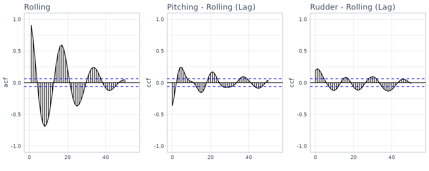
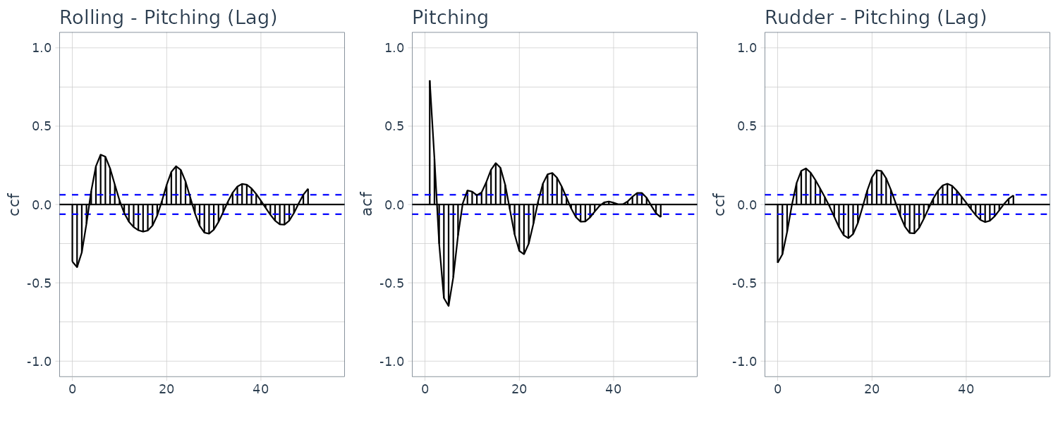
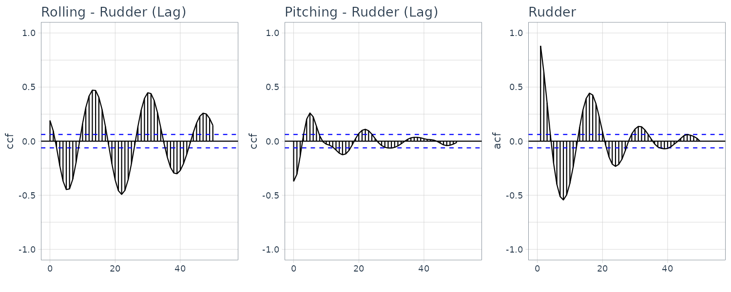
From these figures, it can be seen that the roll rate and the rudder angle fluctuate somewhat periodically. On the other hand, the autocorrelation function of the pitch rate is complicated. Furthermore, the plots in the above figure indicate a strong correlation between the roll rate, \(\textbf{y}_{n}(1)\), and the rudder angle, \(\textbf{y}_{n−k}(3)\). The autocorrelation functions of the roll rate and rudder angle are similar and the cross-correlation \(R_{k}(1, 3)\) between the rudder angle and the roll rate is very high but \(R_{n}(3, 1)\) is rather small. The cross-correlation suggests that rudder angle affects the variation of the roll rate but not vice versa.
Power Spectrum
By means of spectral analysis, we can capture the characteristics of time series by decomposing time series into trigonometric functions at each frequency and by representing the features with the magnitude of each periodic component.
If the autocovariance function \(C_{k}\) rapidly decreases as the lag k increases and satisfies:
\[\begin{aligned} \sum_{k=-\infty}^{\infty}|C_{k}| < \infty \end{aligned}\]Then we can define the Fourier Transform of \(C_{k}\). We define the power spectral density function on frequency \(f\) as:
\[\begin{aligned} p(f) &= \sum_{k = -\infty}^{\infty}C_{k}e^{-2\pi ikf} \end{aligned}\] \[\begin{aligned} -\frac{1}{2} \leq f \leq \frac{1}{2} \end{aligned}\]Because the ACF is an even function and satisfies \(C_{k} = C_{-k}\):
\[\begin{aligned} p(f) &= \sum_{k = -\infty}^{\infty}C_{k}e^{-2\pi ikf}\\ &= \sum_{k = -\infty}^{\infty}C_{k} \mathrm{cos}(2\pi k f) - i \sum_{k = -\infty}^{\infty}C_{k} \mathrm{sin}(2\pi k f)\\ &= \sum_{k = -\infty}^{\infty}C_{k} \mathrm{cos}(2\pi k f) - 0\\ &= C_{0} + 2\sum_{k = 1}^{\infty}C_{k} \mathrm{cos}(2\pi k f) \end{aligned}\]The imaginary part disappears because even function multiply by even function result in an even function. The integral of both sides of the axis result in 0.
Hence, given the power spectrum, we can derive the ACF by taking the inverse Fourier Transform:
\[\begin{aligned} C_{k} &= \int_{-\frac{1}{2}}^{\frac{1}{2}}p(f)e^{2\pi i k f}\ df\\ &= \int_{-\frac{1}{2}}^{\frac{1}{2}}p(f)\mathrm{cos}(2\pi k f)\ df - i\int_{-\frac{1}{2}}^{\frac{1}{2}}p(f)\mathrm{sin}(2\pi k f)\ df\\ &= \int_{-\frac{1}{2}}^{\frac{1}{2}}p(f)\mathrm{cos}(2\pi k f)\ df \end{aligned}\]Note the multiplication of even and odd function results in an odd function and taking integral result in 0.
Ex: Power Spectrum of White Noise
The ACF of a white noise is given by:
\[\begin{aligned} C_{k} &= \begin{cases} \sigma^{2} & k = 0\\ 0 & k \neq 0 \end{cases} \end{aligned}\]Therefore, the power spectrum of a white noise is:
\[\begin{aligned} p(f) &= \sum_{k = -\infty}^{\infty}C_{k}\mathrm{cos}(2\pi k f)\\ &= C_{0}\mathrm{cos}(0)\\ &= \sigma^{2} \end{aligned}\]In this case the power spectrum is a constant number which mean the white noise signal has frequency components across all spectrum.
Example: Power spectrum of an AR model
If a time series is generated by a first-order autoregressive (AR) model:
\[\begin{aligned} y_{n} = \phi y_{n−1} + w_{n} \end{aligned}\]The autocovariance function is given by:
\[\begin{aligned} C_{k} &= \sigma^{2}\frac{\phi^{|k|}}{1 - \phi^{2}} \end{aligned}\]And the power spectrum of this time series can be expressed as:
\[\begin{aligned} p(f) &= \frac{\sigma^{2}}{|1 - \phi e^{-2\pi i f}|^{2}}\\ &= \frac{\sigma^{2}}{1 - 2\phi\textrm{cos}(2\pi f) + \phi^{2}} \end{aligned}\]Note that:
\[\begin{aligned} |1 - \phi e^{-2\pi i f}|^{2} &= (|1 - \phi e^{-2\pi i f}|)^{2}\\ &= (|1 - \phi(\textrm{cos}(2\pi f) + i\textrm{sin}(2\pi f))|)^{2}\\ &= (|1 - \phi\textrm{cos}(2\pi f) + i\phi\textrm{sin}(2\pi f)|)^{2}\\ &= (\sqrt{(1 - \phi\textrm{cos}(2\pi f))^{2} + \phi^{2}\textrm{sin}(2\pi f)^{2}})^{2}\\ &= (1 - \phi\textrm{cos}(2\pi f))^{2} + \phi^{2}\textrm{sin}(2\pi f)\\ &= 1 - 2\phi\textrm{cos}(2\pi f) + \phi^{2}[\textrm{cos}(2\pi f)^{2} + \textrm{sin}(2\pi f)^{2}]\\ &= 1 - 2\phi\textrm{cos}(2\pi f) + \phi^{2} \end{aligned}\]If a time series follows a second-order AR model:
\[\begin{aligned} y_{n} = \phi_{1} y_{n−1} + \phi_{2} y_{n−2} + w_{n} \end{aligned}\]The autocorrelation function satisfies:
\[\begin{aligned} R_{1} &= \frac{\phi_{1}}{1 - \phi_{2}}\\ R_{k} &= \phi_{1}R_{k-1} + \phi_{2}R_{k-2} \end{aligned}\]And the power spectrum can be expressed as:
\[\begin{aligned} p(f) &= \frac{\sigma^{2}}{|1 - \phi_{1}e^{-2\pi i f} - \phi_{2}e^{-4\pi i f}|^{2}}\\ &= \frac{\sigma^{2}}{1 - 2\phi_{1}(1 - \phi_{2})\textrm{cos}(2\pi f) - 2\phi_{2}\textrm{cos}(4\pi f) + \phi_{1}^{2} + \phi_{2}^{2}} \end{aligned}\]Periodogram
Given a time series \(y_{1}, \cdots, y_{N}\), the periodogram is defined by:
\[\begin{aligned} p_{j} &= \sum_{k = -N + 1}^{N - 1}\hat{C}_{k}e^{-2\pi i k f_{j}}\\ &= \hat{C}_{0} + 2\sum_{k = 1}^{N-1}\hat{C}_{k}\mathrm{cos}(2\pi k f_{j}) \end{aligned}\]In the definition of the periodogram, we consider only the natural frequencies defined by:
\[\begin{aligned} f_{j} &= \frac{j}{N} \end{aligned}\] \[\begin{aligned} j &= 0, \cdots, \Big\lfloor \frac{N}{2} \Big\rfloor \end{aligned}\]Where \(\lfloor \frac{N}{2} \rfloor\) denotes the maxium integer which does not exceed \(\frac{N}{2}\).
The sample spectrum is an extension of periodogram by extending the domain to the continuous interval \([-0.5, 0.5]\) (note the frequency is now a continuous value and not just natural frequencies):
\[\begin{aligned} \hat{p}(f) &= \sum_{k = -N + 1}^{N-1}\hat{C}_{k}e^{-2\pi ik f} \end{aligned}\] \[\begin{aligned} -\frac{1}{2} \leq f \leq \frac{1}{2} \end{aligned}\]In other words, the periodogram is obtained from the sample spectrum by restricting its domain to the natural frequencies.
The following relation holds between the sample spectrum and the sample autocovariance function:
\[\begin{aligned} \hat{C}_{k} &= \int_{-\infty}^{\infty}\hat{p}(f)e^{2\pi ik f}\ df \end{aligned}\] \[\begin{aligned} k &= 0, \cdots, N-1 \end{aligned}\]The sample spectrum are asymptotically unbiased and satisfy:
\[\begin{aligned} \lim_{N \rightarrow \infty}E[\hat{p}(f)] &= p(f) \end{aligned}\]This means that at each frequency f, the expectation of the sample spectrum converges to the true spectrum as the number of data increases. However, it does not imply the consistency of \(\hat{p}(f)\), that is, the sample spectrum does not necessarily converge to the true spectrum \(p(f)\) as the number of data increases. We can show that the variance of the periodogram is a constant, independent of the sample size N. Thus the periodogram cannot be a consistent estimator.
Smoothing the Periodogram (Raw Spectrum)
Turns out if we sum to a fix \(L\) rather than the size of the sample, the estimator converges to the true spectrum as \(N \rightarrow \infty\):
\[\begin{aligned} p_{j} &= \hat{C}_{0} + 2 \sum_{k = 1} ^{L-1}\hat{C}_{k}\mathrm{cos}(2\pi k f_{j})\\ \end{aligned}\]Averaging and Smoothing of the Periodogram
In this section, we shall consider a method of obtaining an estimator that converges to the true spectrum as the data length n increases. We define \(p_{j}\):
\[\begin{aligned} p_{j} &= \hat{C}_{0} + 2 \sum_{k=1}^{L-1}\hat{C}_{k}\textrm{cos}(2\pi k f_{j}) \end{aligned}\] \[\begin{aligned} f_{j} &= \frac{j}{2L} \end{aligned}\] \[\begin{aligned} j &= 0, \cdots, L \end{aligned}\]Where \(L\) is an aribitrary integer smaller than N. The above is called the raw spectrum.
Recall if we use \(N\) instead:
\[\begin{aligned} p_{j} &= \hat{C}_{0} + 2 \sum_{k=1}^{N-1}\hat{C}_{k}\textrm{cos}(2\pi k f_{j}) \end{aligned}\] \[\begin{aligned} f_{j} &= \frac{j}{N} \end{aligned}\] \[\begin{aligned} j &= 0, \cdots, \Big\lfloor \frac{N}{2} \Big\rfloor \end{aligned}\]In the definition of the periodogram, the sample autocovariances are necessary up to the lag N − 1. However, by just using the first L − 1 autocovariances for properly fixed lag L, the raw spectrum converges to the true spectrum as the data length (N) increases. On the assumption that the data length N increases according to \(N = lL\), computing the raw spectrum with the maximum lag L − 1 is equivalent to applying the following procedures:
- Divide the time series \(y_{1}, \cdots, y_{n}\) into \(\frac{N}{L}\) sub-series of length L.
- Obtain a periodogram \(p_{j}^{(i)}\) from each \(\frac{N}{L}\) subseries.
- The averaged periodogram is obtained by:
Even though the variance of each \(p_{j}^{(i)}\) does not change even if N increases, the variance of \(p_{j}\) becomes \(\frac{1}{l}\) of \(p_{j}^{(i)}\). Therefore, the variance of \(p_{j}\) converges to 0 as the number of data points N or \(l\) increases to infinity.
Here, note that the raw spectrum does not exactly agree with the averaged periodogram:
\[\begin{aligned} p_{j} &= \hat{C}_{0} + 2\sum_{k=1}^{L-1}\hat{C}_{k}\mathrm{cos}(2\pi k f_{j}) \end{aligned}\] \[\begin{aligned} p_{j} &= \frac{L}{N}\sum_{i=1}^{\frac{N}{L}}p_{j}^{(i)} \end{aligned}\]And sometimes it might happen that \(p_{j} < 0\). To prevent this situation and to guarantee the positivity of \(p_{j}\), we need to compute \(p_{j}\) by the second equation.
However in actual computation, the raw spectrum is smoothed by using the spectral window. That is, for a given spectral window \(W_{k}\), \(i = 0, \pm1, \cdots, \pm m\), an estimate of the spectrum is obtained by:
\[\begin{aligned} \hat{p}_{j} &= \sum_{i=-m}^{m}W_{i}p_{j-i} \end{aligned}\] \[\begin{aligned} j = 0, 1, \cdots, \Big\lfloor \frac{L}{2} \Big\rfloor \end{aligned}\]Where:
\[\begin{aligned} p_{-j} &= p_{j}\\ p_{\lfloor \frac{L}{2} \rfloor + i} &= p_{\lfloor \frac{L}{2} \rfloor - i} \end{aligned}\]By properly selecting a spectral window, we can obtain an optimal estimate of the spectrum that is always positive and with smaller variance.
Computation of the Periodogram by Fast Fourier Transform
Because computing the periodogram require the computation of Fourier transform of the sample autocovariance function:
\[\begin{aligned} p_{j} &= \hat{C}_{0} + 2\sum_{k = 1}^{N-1}\hat{C}_{k}\mathrm{cos}(2\pi k f_{j}) \end{aligned}\]And the computation of the sample ACF requires \(\frac{N^{2}}{2}\) operations, it would be more efficient to apply the FFT directly to the time series.
The FFT, \(X_{j}\), is obtained by:
\[\begin{aligned} X_{j} &= \sum_{n=1}^{N}y_{n}e^{-2\pi(n-1)\frac{j}{N}}\\ &= \sum_{n=1}^{N}y_{n}\textrm{cos}\frac{2\pi(n-1)j}{N} - i\sum_{n=1}^{N}y_{n}\textrm{sin}\frac{2\pi(n-1)j}{N}\\ &= \text{FC}_{j} - i\text{FS}_{j} \end{aligned}\] \[\begin{aligned} j &= 0, \cdots, \frac{N}{L} \end{aligned}\]Then the periodogram is obtained by:
\[\begin{aligned} p_{j} &= \frac{|X_{j}|^{2}}{N}\\ &= \frac{1}{N}\Big|\sum_{n=1}^{N}y_{n}e^{-2\pi i (n-1)\frac{j}{N}}\Big|^{2}\\ &= \frac{\text{FC}_{j}^{2} + \text{FS}_{j}^{2}}{N} \end{aligned}\]It can be shown that the above is equivalent to:
\[\begin{aligned} p_{j} &= \hat{C}_{0} + 2\sum_{k = 1}^{N-1}\hat{C}_{k}\mathrm{cos}(2\pi k f_{j}) \end{aligned}\] \[\begin{aligned} p_{j} &= \frac{1}{N}\Big|\sum_{n=1}^{N}y_{n}e^{-2\pi i (n-1)\frac{j}{N}}\Big|^{2}\\ &= \frac{1}{N}\Big|\sum_{n=1}^{N}y_{n}\textrm{cos}\frac{2\pi(n-1)j}{N} - i\sum_{n=1}^{N}y_{n}\textrm{sin}\frac{2\pi(n-1)j}{N}\Big|^{2}\\ &= \frac{y_{n}}{N}\Big(\sum_{n=1}^{N}\textrm{cos}\frac{2\pi(n-1)j}{N} - i\sum_{n=1}^{N}\textrm{sin}\frac{2\pi(n-1)j}{N}\Big)\Big(\sum_{n=1}^{N}\textrm{cos}\frac{2\pi(n-1)j}{N} + i\sum_{n=1}^{N}\textrm{sin}\frac{2\pi(n-1)j}{N}\Big)\\ &= \frac{1}{N}\Big(\sum_{n=1}^{N}e^{-2\pi i(n-1)\frac{j}{N}}y_{n}\Big)\Big(\sum_{n=1}^{N}e^{2\pi i(n-1)\frac{j}{N}}y_{n}\Big)\\ &= \frac{1}{N}\sum_{s=1}^{N}\sum_{t=1}^{N}e^{-2\pi i (s -1 - (t - 1))\frac{j}{N}}y_{s}y_{t}\\ &= \frac{1}{N}\sum_{s=1}^{N}\sum_{t=1}^{N}e^{-2\pi i (s - t)\frac{j}{N}}y_{s}y_{t}\\ &= \sum_{k = -N+1}^{N-1}\hat{C}_{k}e^{-2\pi i k \frac{j}{N}} \end{aligned}\]For a time series of general length, i.e., not expressible in the form of \(N = 2^{l}\), is to apply the FFT after modifying the time series by adding \((2{l} − N)\) zeros behind the data, to make it of length \(N' = 2^{l}\). Then we obtain the sample spectrum for the frequencies:
\[\begin{aligned} f_{j} &= \frac{j}{N'}\\ \end{aligned}\] \[\begin{aligned} j &= 0, \cdots, \frac{N'}{2} \end{aligned}\]Therefore, if \(N \neq 2^{l}\), the periodogram obtained using the FFT is evaluated at different frequencies from those of the periodogram obtained directly. These differences are not so crucial when the true spectrum is continuous. However, if the true spectrum contains line spectra or sharp peaks, the two methods might yield quite different results.
For example, we generate the following time series with 2 line spectra:
\[\begin{aligned} y_{n} &= \textrm{cos}\frac{2\pi n}{10} + \textrm{cos}\frac{2\pi n}{4} + w_{n} \end{aligned}\] \[\begin{aligned} N = 400 \end{aligned}\] \[\begin{aligned} w_{n} &\sim N(0, 0.01) \end{aligned}\]dat <- tsibble(
t = 1:400,
r = rnorm(400, sd = 0.01),
y = rep(0, 400),
index = t
)
for (i in 1:nrow(dat)) {
dat$y[i] <- cos(2 * pi * i / 10) +
cos(2 * pi * i / 4) +
dat$r[i]
}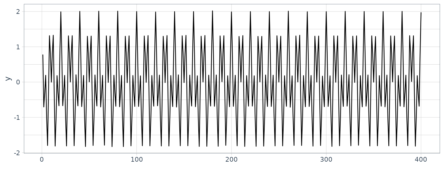
Contrasting the original FFT and padded FFT:
fs <- nrow(dat)
dat1 <- tibble(
  fft = Mod(fft(dat$y))[1:(fs / 2)],
  f = seq(0, 0.5, length.out = fs / 2)
)

diff <- 512 - fs

dat2 <- tibble(
  fft = Mod(
    fft(
      c(dat$y, rep(0, diff))
    )
  )[1:(fs / 2)],

  f = seq(0, 0.5, length.out = fs / 2)
)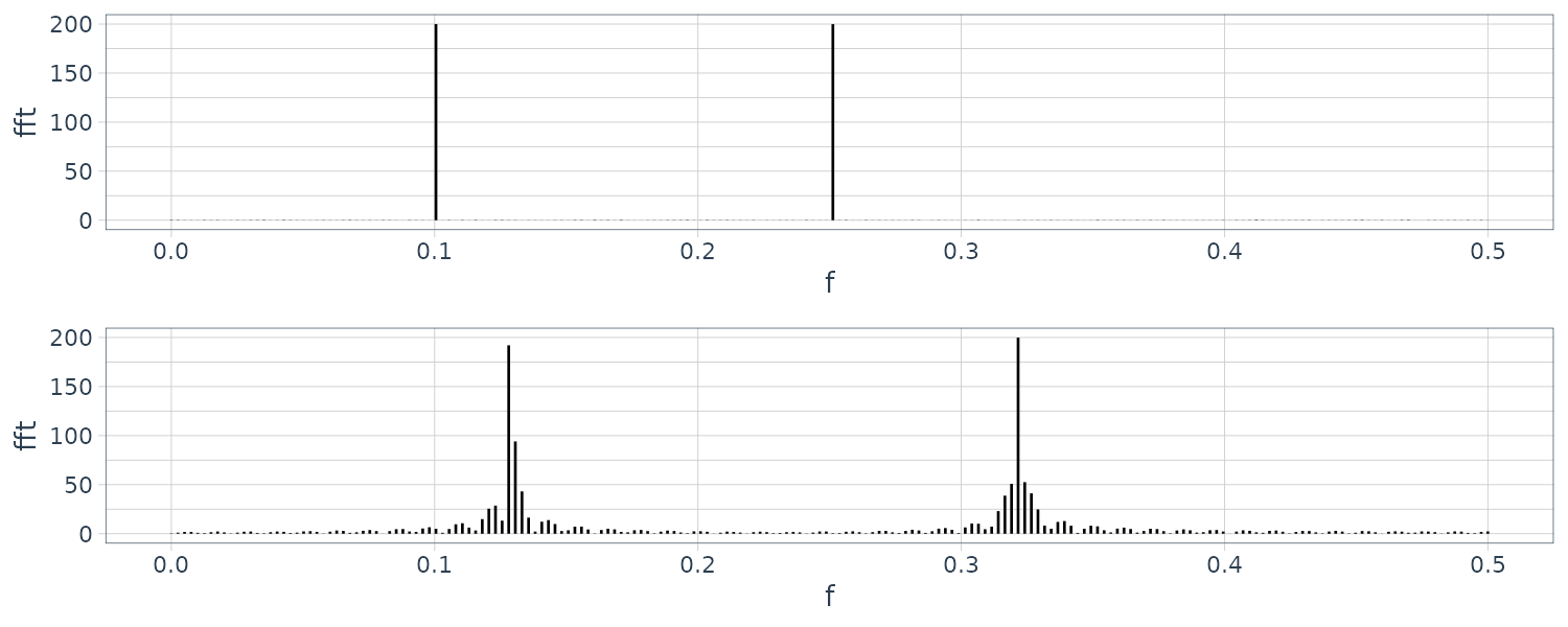
In this case, the second periodogram looks quite different from the first periodogram, because the frequencies to be calculated for the second periodogram have deviated from the position of the line spectrum.
However for the HAKUSAN yaw rate data:
dat <- HAKUSAN |>
  filter(key == "YawRate")

fs <- nrow(dat)
dat1 <- tibble(
  fft = Mod(fft(dat$value))[1:(fs / 2)],
  f = seq(0, 0.5, length.out = fs / 2)
)
diff <- 1024 - fs
dat2 <- tibble(
  fft = Mod(
    fft(
      c(dat$value, rep(0, diff))
    )
  )[1:(fs / 2)],
  f = seq(0, 0.5, length.out = fs / 2)
)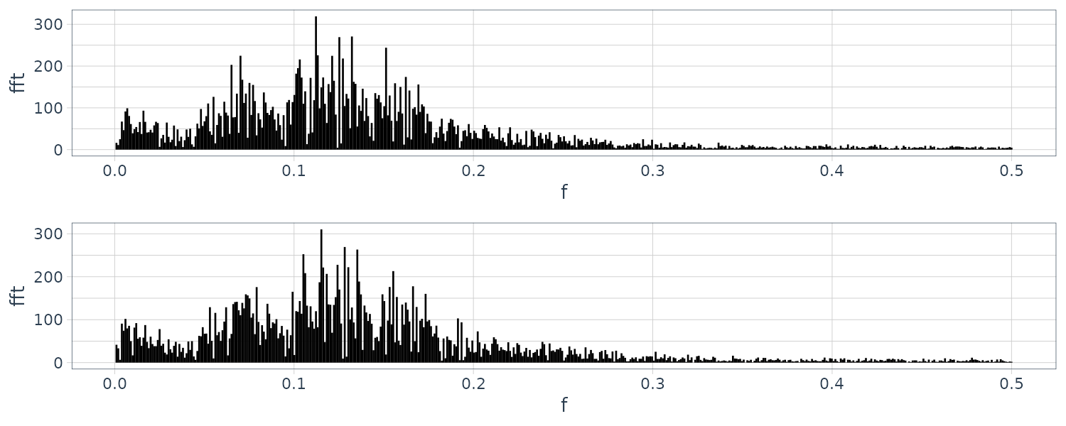
This example shows that if the spectrum is continuous and does not contain any line spectra, the periodogram obtained by using FFT after padding zeros behind the data is similar to the periodogram obtained using the original definition.
Let us now investigate each dataset acf and periodogram:
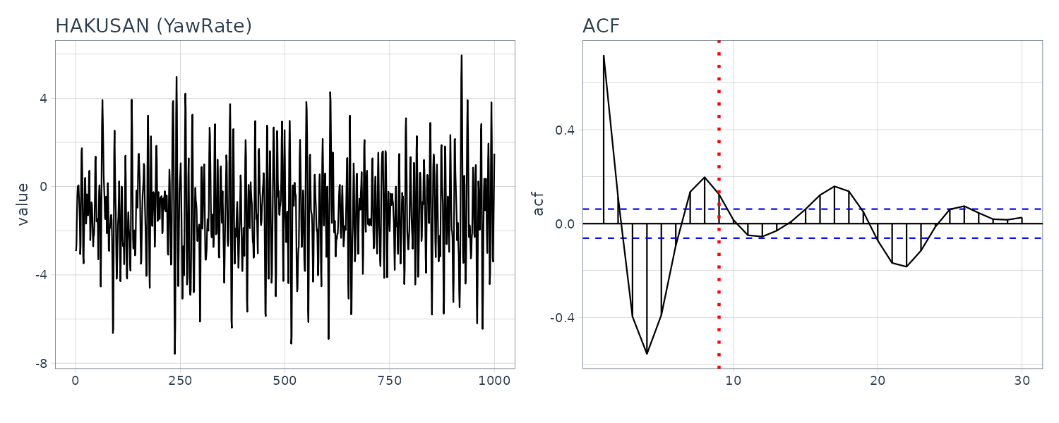
HAKUSAN
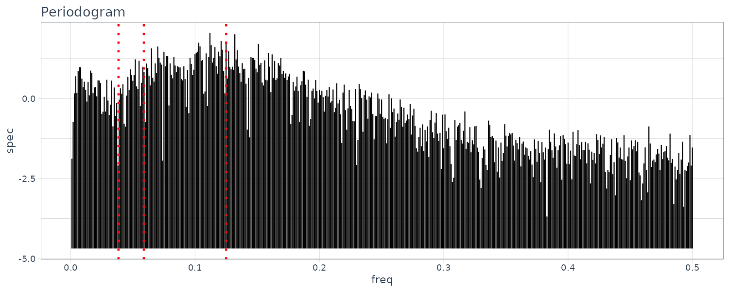
When we can see the sample ACF decaying to 0 with a possible cycle of 8 (see dotted lines). The periodogram also agree with a peak at 0.125.
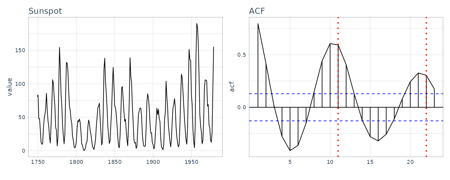
Sunspot
The peaks of the sample autocorrelation function repeatedly appear at an almost eleven-year cycle corresponding to the approximate eleven-year cycle of the sunspot number data and the amplitude of the sample autocorrelation gradually decreases as the lag increases. Also evident on the periodogram at frequency 0.917 which correspond to 11y.
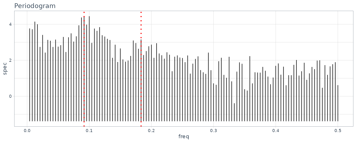
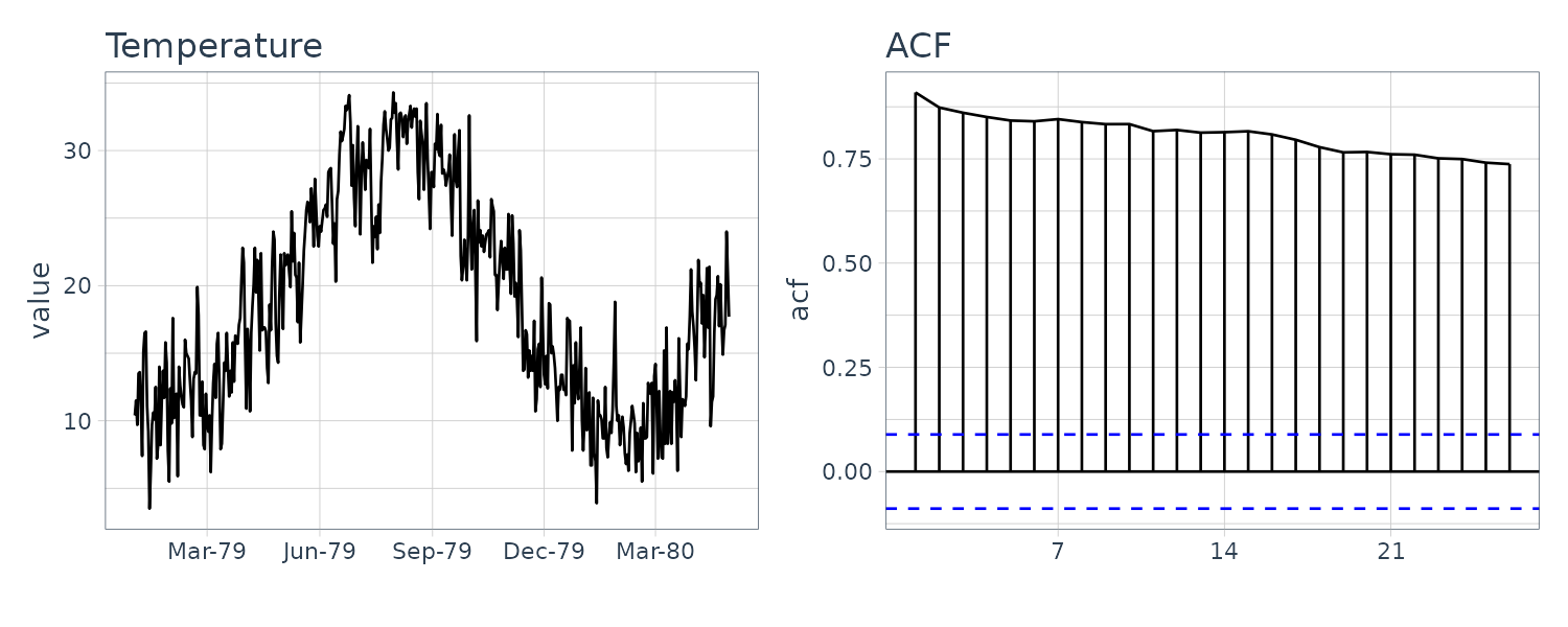
Temperature
The ACF decay really slowly due to a annual trend and the full cycle is not apparent in the plot.
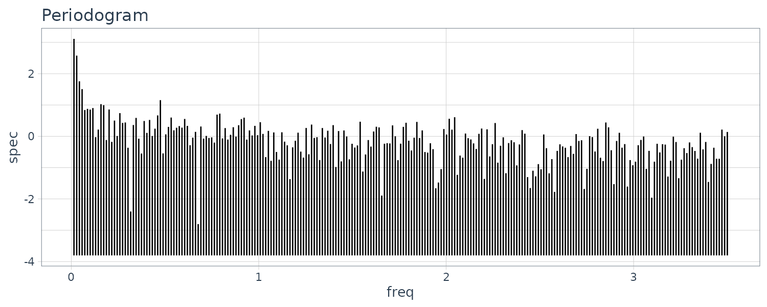
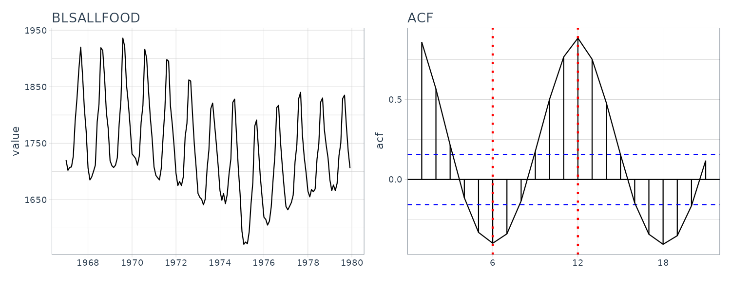
BLSALLFOOD
A one-year cycle in the sample autocorrelation function is seen corresponding to the semi-annual and annual cycle of the time series. However, the amplitude of the sample autocorrelation function decreases more slowly than those of the Sunspot due to the presence of a trend. The periodogram is showing frequency of integer multiples close to 1y. These are consider higher harmonics of the nonlinear harmonics.
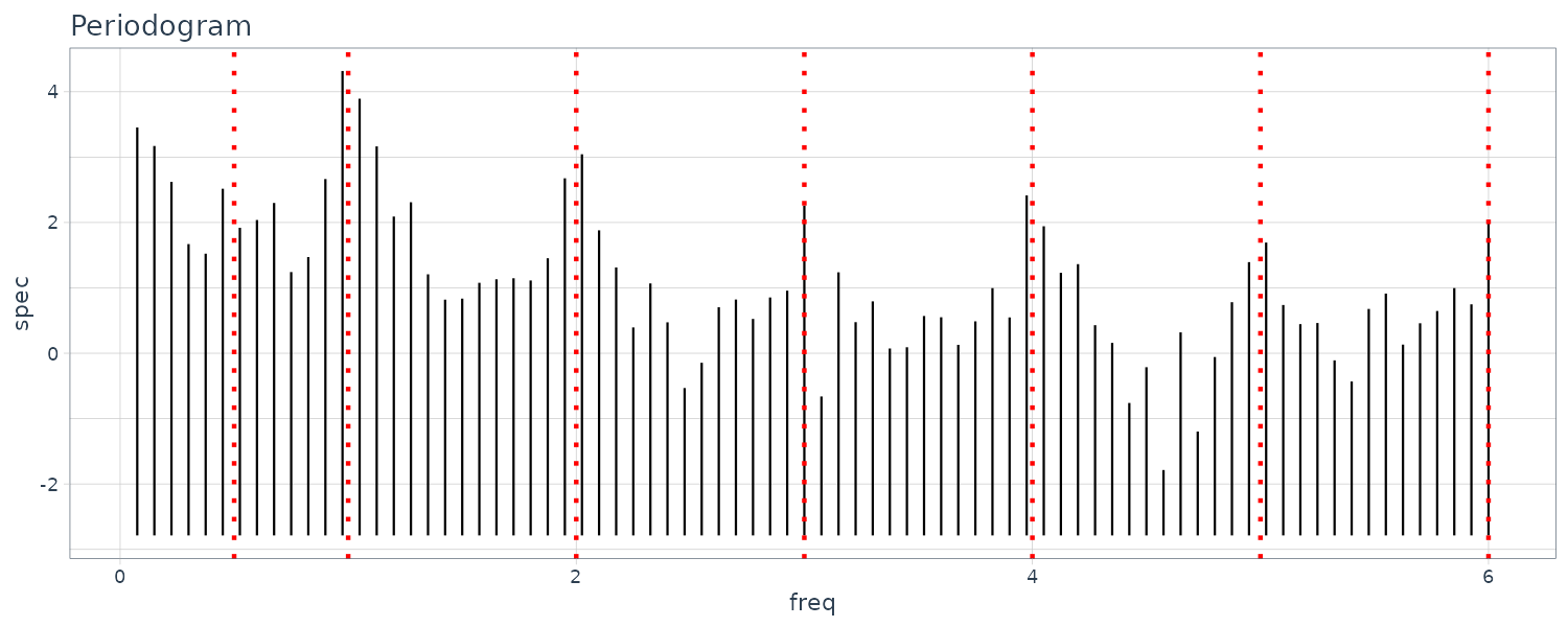
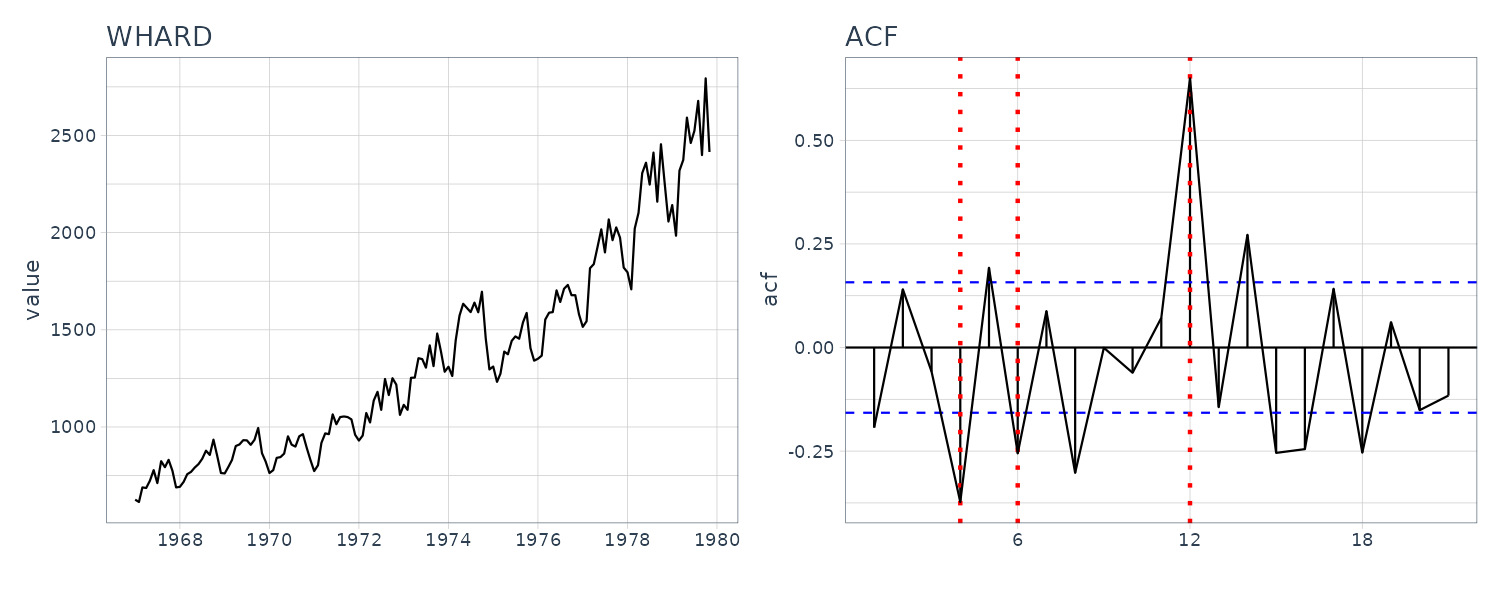
WHARD
Uptrend with amplitude growing. For the ACF and periodogram, we compute it on the log difference instead. We can see a cycle on the 4, 6, and 12 weeks.
MYE1F
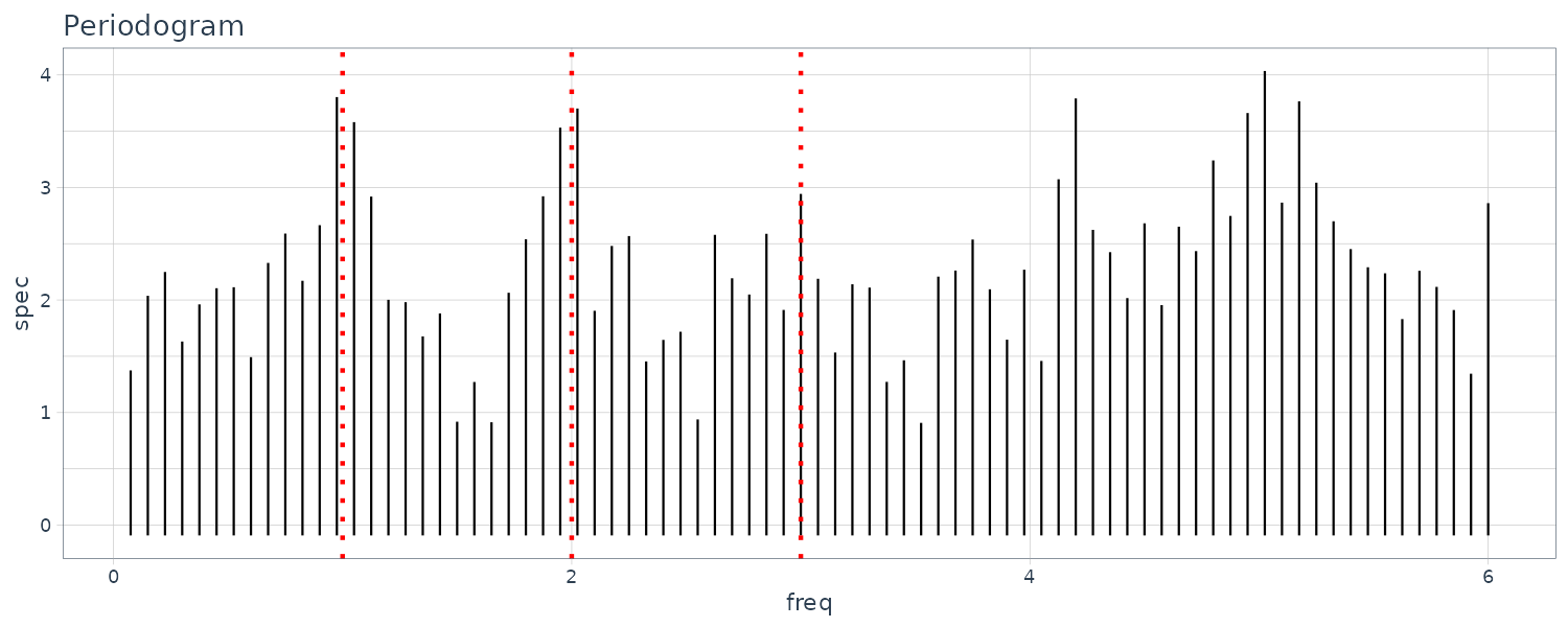
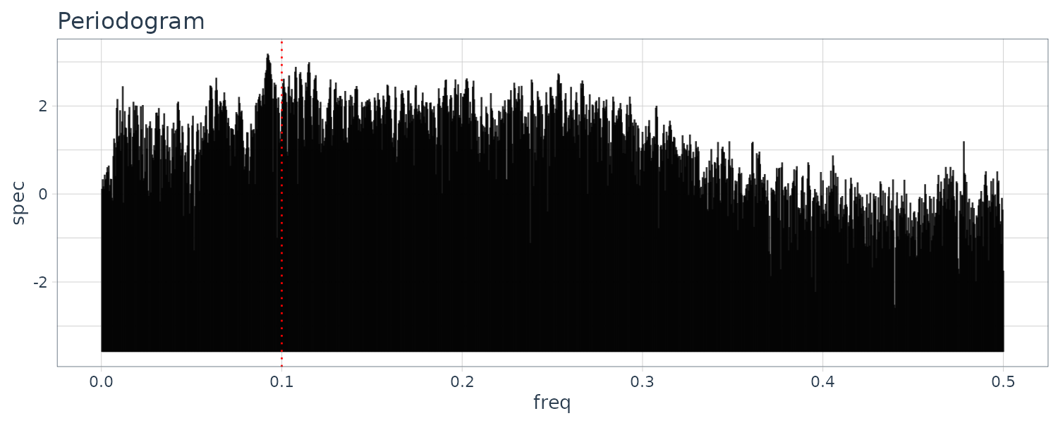
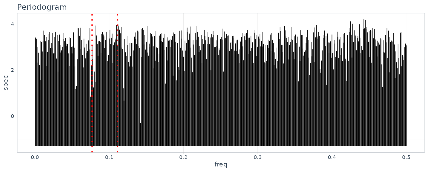
The fluctuation of the sample autocorrelation function continues for a considerably long time with an approximate 10-second cycle after a sudden reduction in the amplitude. The periodogram shows a peak at frequency 0.1.
SPX
Similar to WHARD, for the ACF and periodogram, we compute on the log difference. From the periodogram, we can’t see any prominent peaks and a possible 9, 13 day cycle.
Statistical Modeling
In the statistical analysis of time series, measurements of a phenomenon with uncertainty are considered to be the realization of a random variable that follows a certain probability distribution. if a probability distribution or a density function is given, we can generate data that follow the distribution.
On the other hand, in statistical analysis, when data \(y_{1}, \cdots, y_{N}\) are given, they are considered to be realizations of a random variable Y. That is, we assume a random variable Y underlying the data and consider the data as realizations of that random variable. Here, the density function g(y) defining the random variable is called the true model. Since this true model is usually unknown for us, it is necessary to estimate the probability distribution from the data. Here, the density function estimated from data is called a statistical model and is denoted by f(y).
Probability Distributions and Statistical Models
In statistical analysis, various distributions are used to model characteristics of the data. Typical density functions are as follows:
1) Normal Distribution
\[\begin{aligned} g(x) &= \frac{1}{\sqrt{2\pi\sigma^{2}}}e^{-\frac{(x - \mu)^{2}}{2\sigma^{2}}} \end{aligned}\] \[\begin{aligned} -\infty < x < \infty \end{aligned}\]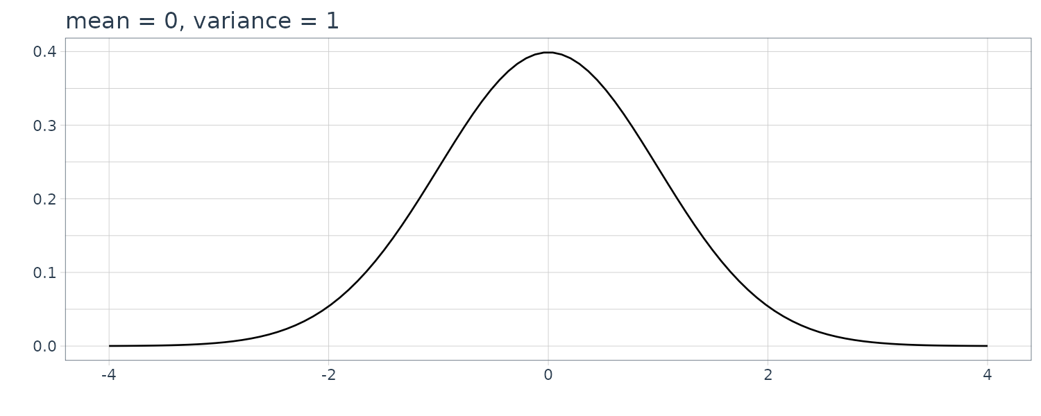
The above is called a normal distribution or a Gaussian distribution with the mean \(\mu\) and the variance \(\sigma^{2}\), and is denoted by \(N(\mu, \sigma^{2})\). In particular, N(0, 1) is called the standard normal distribution.
2) Cauchy Distribution
\[\begin{aligned} g(x) &= \frac{\tau}{\pi[(x - \mu)^{2} + \tau^{2}]} \end{aligned}\] \[\begin{aligned} -\infty < x < \infty \end{aligned}\]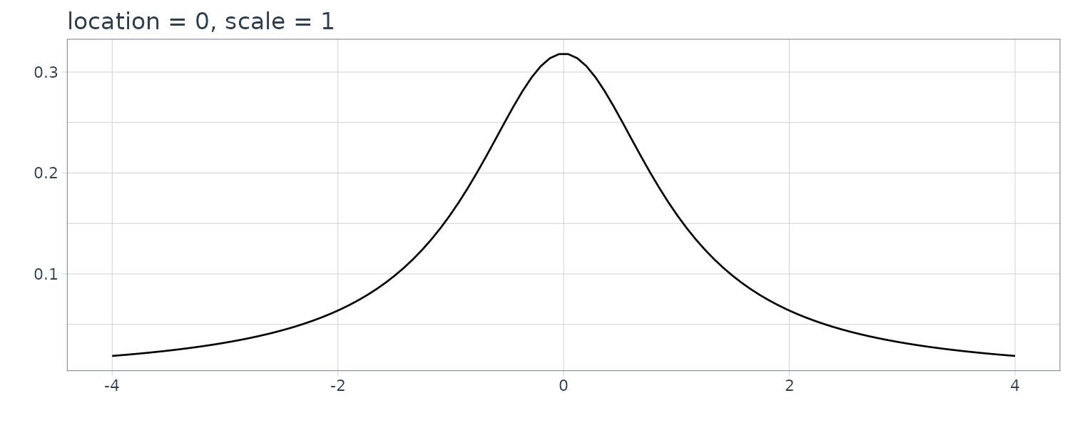
The above is called a Cauchy distribution. \(\mu\) and \(τ^{2}\) are called the location parameter and the dispersion parameter, respectively. Note that the square root of dispersion parameter, \(\tau\), is called the scale parameter.
3) Pearson Family of Distributions
\[\begin{aligned} g(x) &= \frac{c}{[(x - \mu)^{2} + \tau^{2}]^{b}} \end{aligned}\] \[\begin{aligned} -\infty < x < \infty \end{aligned}\]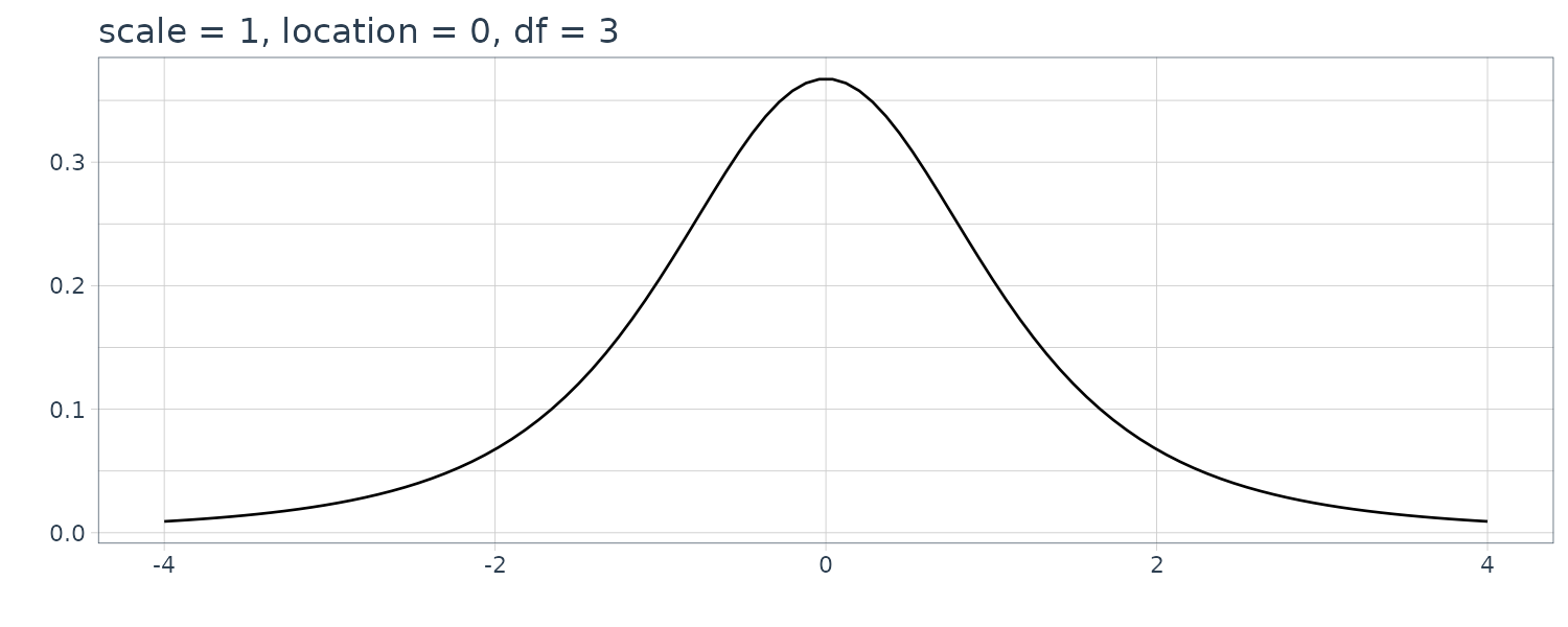
The above is called the (type VII) Pearson family of distributions with central parameter \(\mu\), dispersion parameter \(\tau^{2}\) and shape parameter b. Here c is a normalizing constant given by:
\[\begin{aligned} c = \frac{\tau^{2b-1}\Gamma(b)}{\Gamma(b - \frac{1}{2})\Gamma(\frac{1}{2})} \end{aligned}\]This distribution agrees with the Cauchy distribution for \(b = 1\). Moreover, if \(b = \frac{k + 1}{2}\) with a positive integer \(k\), it is called the t-distribution with k degrees of freedom.
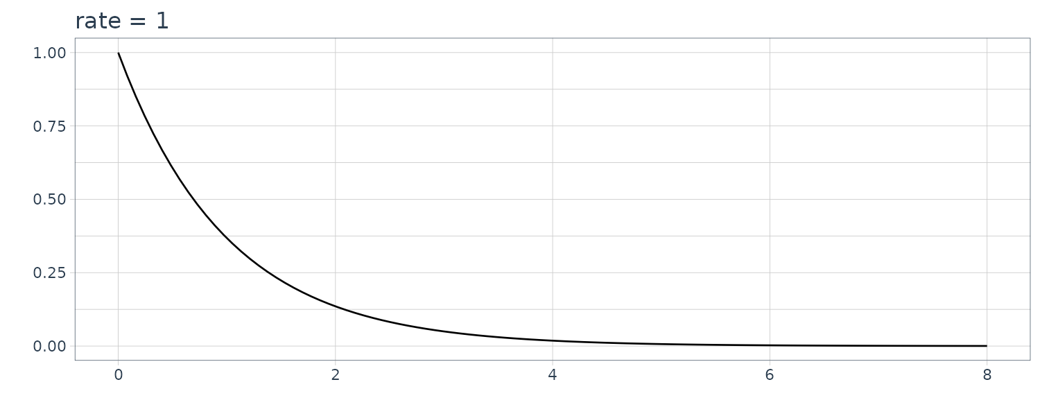
4) Exponential Distribution
\[\begin{aligned} g(x) &= \begin{cases} \lambda e^{-\lambda x} & x \geq 0\\ 0 & x < 0 \end{cases} \end{aligned}\]The above is called the exponential distribution. The mean and the variance of the exponential distribution are given by \(\frac{1}{\lambda}\) and \(\frac{1}{λ^{2}}\), respectively.
5) \(\chi^{2}\)-Distribution
\[\begin{aligned} g(x) &= \begin{cases} \frac{1}{2^{\frac{k}{2}}\Gamma(\frac{k}{2})}e^{-\frac{x}{2}}x^{\frac{k}{2}-1} & x \geq 0\\ 0 & x < 0 \end{cases} \end{aligned}\]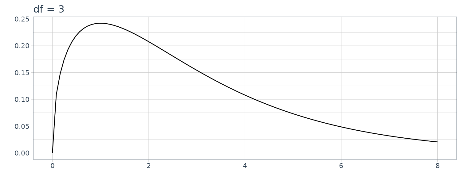
The above is called the \(\chi^{2}\) distribution with \(k\) degrees of freedom. Especially, for \(k = 2\), it becomes an exponential distribution. The mean and the variance of the \(\chi^{2}\) distribution are \(k\) and \(2k\), respectively. The sum of the square of \(k\) Gaussian random variables follows the \(\chi^{2}\) distribution with \(k\) degrees of freedom.
\[\begin{aligned} -\infty < x < \infty \end{aligned}\]6) Double Exponential (Laplace) Distribution
\[\begin{aligned} g(x) &= e^{x - e^{x}} \end{aligned}\] \[\begin{aligned} -\infty < x < \infty \end{aligned}\]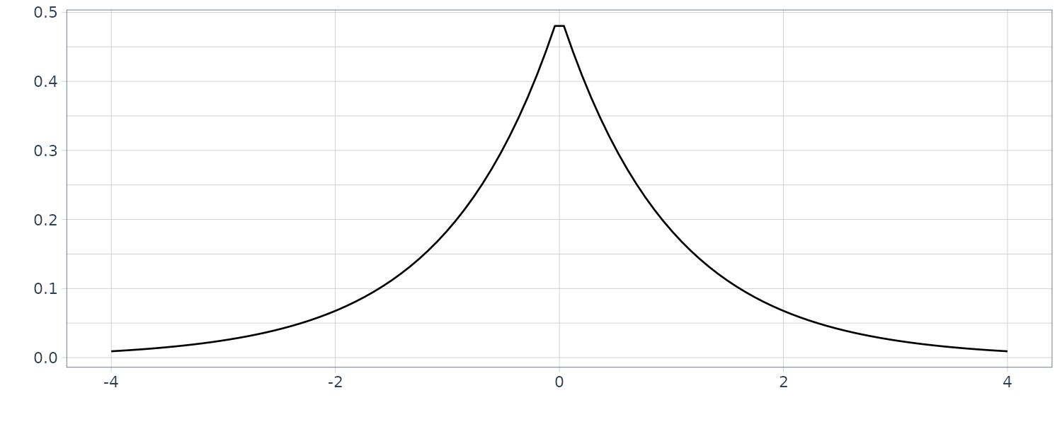
The above is called the Double Exponential (Laplace) distribution. The mean and the vari ance of this distribution are \(-\xi\) and \(\frac{\pi^{2}}{6}\), respectively, where \(\xi = 0.577224\) is the Euler constant. The logarithm of the exponential random variable follows the double exponential distribution.
7) Uniform Distribution
\[\begin{aligned} g(x) &= \begin{cases} \frac{1}{b-a} & a \leq x < b\\ 0 & \text{otherwise} \end{cases} \end{aligned}\]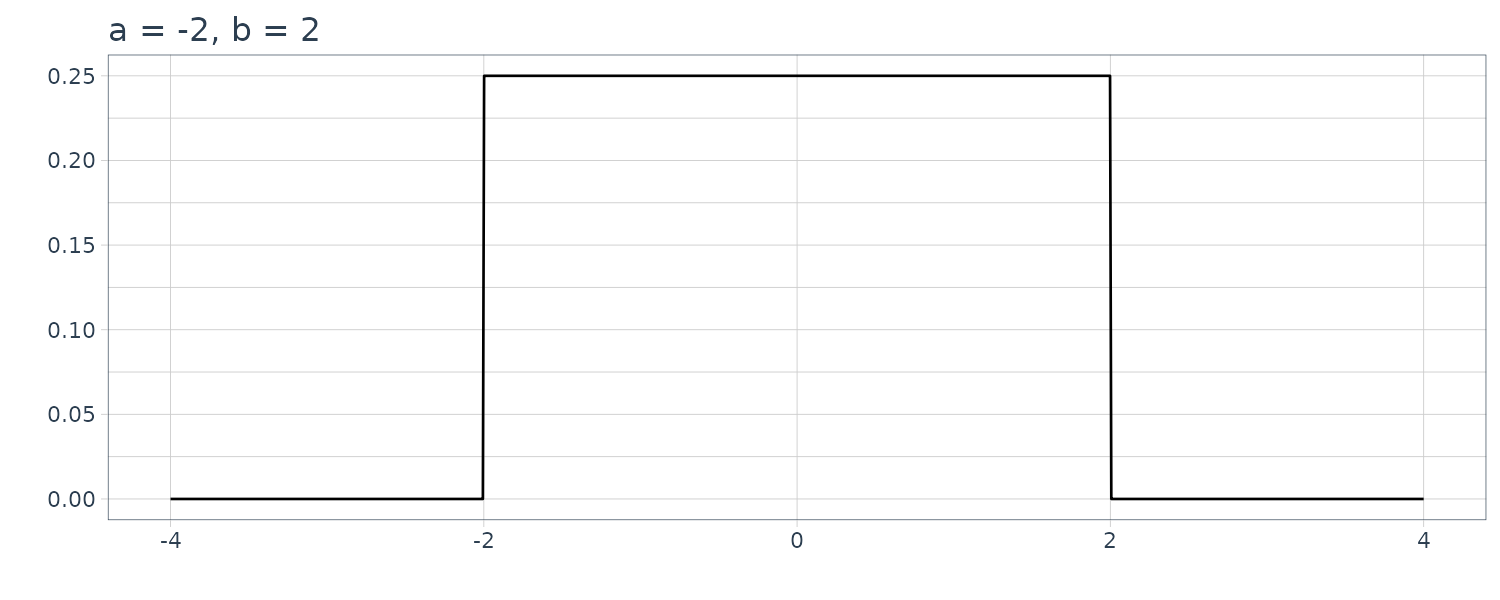
The above is called the uniform distribution over \([a, b)\). The mean and the variance of the uniform distribution are \(\frac{a+b}{2}\) and \(\frac{(b−a)^{2}}{12}\), respectively.
In ordinary statistical analysis, the probability distribution is sufficient to characterize the data, whereas for time series data, we have to consider the joint distribution \(f(y_{1}, \cdots, y_{N})\). If the time series is stationary, we can express the model using a multidimensional normal distribution with mean vector:
\[\begin{aligned} \begin{bmatrix} \hat{\mu}\\ \vdots\\ \hat{\mu} \end{bmatrix} \end{aligned}\]And variance covariance matrix:
\[\begin{aligned} \textbf{C} &= \begin{bmatrix} \hat{C}_{0} & \hat{C}_{1} & \cdots & \hat{C}_{N-1}\\ \hat{C}_{1} & \hat{C}_{0} & \cdots & \hat{C}_{N-2}\\ \vdots & \vdots & \ddots & \vdots\\ \hat{C}_{N-1} & \hat{C}_{N-2} & \cdots & \hat{C}_{0} \end{bmatrix} \end{aligned}\]This model can express an arbitrary Gaussian stationary time series very flexibly. However, it cannot achieve an efficient expression of the information contained in the data since it requires the estimation of N +1 unknown parameters, \(\hat{C}_{0}, \cdots, \hat{C}_{N-1}, \hat{\mu}\). We will show later how to reduce the number of parameters.
K-L Information and Entropy Maximization Principle
It is assumed that a true model generating the data is g(y) and that f(y) is an approximating statistical model. In statistical modeling, we aim at building a model f(y) that is “close” to the true model g(y). To achieve this, it is necessary to define a criterion to evaluate the goodness of the model f(y) objectively.
The book uses the Kullback-Leibler information:
\[\begin{aligned} I(g; f) &= E_{Y}\Bigg[\log \frac{g(Y)}{f(Y)}\Bigg]\\ &= \int_{-\infty}^{\infty}\log \frac{g(y)}{f(y)}g(y)\ dy \end{aligned}\]Here, \(E_{Y}\) denotes the expectation with respect to the true density function g(y) and the integral applies to a model with a continuous probability distribution. This K-L information has the following properties:
\[\begin{aligned} I(g; f) &\geq 0 \end{aligned}\] \[\begin{aligned} I(g; f) &= 0 \iff g(y) = f(y) \end{aligned}\]The negative of the K-L information is called the generalized (or Boltzmann) entropy:
\[\begin{aligned} B(g; f) &= -I(g; f) \end{aligned}\]The smaller the value of the K-L information, the closer the probability distribution f (y) is to the true distribution g(y). In statistical modeling, the strategy of constructing a model so as to maximize the entropy \(B(g; f)\) is referred to as the entropy maximization principle.
Example: K-L information of a normal distribution model
Consider the case where both the true model, g(y), and the approximate model, f (y), are normal distributions defined by:
\[\begin{aligned} g(y|\mu, \sigma^{2}) &= \frac{1}{\sqrt{2\pi \sigma^{2}}}e^{-\frac{(y - \mu)^{2}}{2\sigma^{2}}}\\ g(y|\xi, \tau^{2}) &= \frac{1}{\sqrt{2\pi \sigma^{2}}}e^{-\frac{(y - \xi)^{2}}{2\tau^{2}}} \end{aligned}\]And the KL information is given by:
\[\begin{aligned} I(g; f) &= E_{Y}\Big[\log \frac{g(y)}{f(y)}\Big]\\ &= \frac{1}{2}\Big[\log \frac{\tau^{2}}{\sigma^{2}} - \frac{E_{Y}[(y - \mu)]^{2}}{\sigma^{2}} + \frac{E_{Y}[(y - \xi)]^{2}}{\tau^{2}}\Big]\\ &= \frac{1}{2}\Big[\log \frac{\tau^{2}}{\sigma^{2}} - 1 + \frac{\sigma^{2} + (\mu - \xi)^{2}}{\tau^{2}}\Big] \end{aligned}\]For example:
\[\begin{aligned} g(y) &\sim N(0, 1) \end{aligned}\] \[\begin{aligned} f(x) &\sim N(0.1, 1.5) \end{aligned}\]Then:
\[\begin{aligned} I(g; f) &= \frac{1}{2}\times \Big(\log(1.5) - 1 + \frac{1.01}{1.5}\Big)\\ &= 0.03940 \end{aligned}\]The K-L information is easily calculated, if both g and f are normal distributions. However, for general distributions g and f, it is not always possible to compute \(I(g; f)\) analytically. Therefore, in general, to obtain the K-L information, we need to resort to numerical computation like numerical integration over \([x_{0}, x_{k}]\) using the trapezoidal rule for example:
\[\begin{aligned} \hat{I}(g; f) &= \frac{\Delta x}{2}\sum_{i=1}^{k}h(x_{i}) + h(x_{i-1}) \end{aligned}\]Where k is the number of nodes and:
\[\begin{aligned} x_{0} &= -x_{k} \end{aligned}\] \[\begin{aligned} x_{i} &= x_{0} + (x_{k} - x_{0})\frac{i}{k} \end{aligned}\] \[\begin{aligned} h(x) &= g(x)\log\frac{g(x)}{f(x)} \end{aligned}\] \[\begin{aligned} \Delta x &= \frac{x_{k} - x_{0}}{k} \end{aligned}\]Estimation of the K-L Information and the Log-Likelihood
In an actual situation, we do not know the true distribution g(y), but instead we can obtain the data \(y_{1}, \cdots, y_{N}\) generated from the true distribution. Hereafter we consider the method of estimating the K-L information of the model f(y) by assuming that the data \(y_{1}, \cdots, y_{N}\) are independently observed from g(y).
As a first step, the K-L information can be decomposed into two terms as:
\[\begin{aligned} I(g; f) &= E_{Y}[\log g(Y)] - E_{Y}[\log f(Y)] \end{aligned}\]Although the first term on the right-hand side of the above equation cannot be computed unless the true distribution g(y) is given, it can be ignored because it is a constant, independent of the model f(y). Therefore, a model that maximizes the second term on the right-hand side is considered to be a good model. This second term is called expected log-likelihood. For a continuous model with density function f (y), it is expressible as:
\[\begin{aligned} E_{Y}[\log f(Y)] &= \int \log f(y)g(y)\ dy \end{aligned}\]Unfortunately, the expected log-likelihood still cannot be directly calculated when the true model g(y) is unknown. However, because data \(y_{n}\) is generated according to the density function g(y), due to the law of large numbers:
\[\begin{aligned} \lim_{N\rightarrow \infty}\frac{1}{N}\sum_{n=1}^{N}\log f(y_{n}) &= E_{Y}\log f(Y) \end{aligned}\]Therefore, by maximizing the left term, \(\sum_{n=1}^{N}\log f(y_{n})\), instead of the original criterion \(I(g; f)\), we can approximately maximize the entropy.
When the observations are obtained independently, the following are the log-likelihood and likelihood:
\[\begin{aligned} l &= \sum_{n=1}^{N}\log f(y_{n}) \end{aligned}\] \[\begin{aligned} L &= \prod_{n=1}^{N}f(y_{n}) \end{aligned}\]For models used in time series analysis, the assumption that the observations are obtained independently, does not usually hold. For such a general situation, the likelihood is defined by using the joint distribution of \(y_{1}, \cdots, y_{N}\) as:
\[\begin{aligned} L &= f(y_{1}, \cdots, y_{N}) \end{aligned}\] \[\begin{aligned} l &= \log L\\ &= \log f(y_{1}, \cdots, y_{N}) \end{aligned}\]If a model contains a parameter \(\boldsymbol{\theta}\) and its distribution can be expressed as \(f(y) = f(y\mid \boldsymbol{\theta})\), the log-likelihood l can be considered a function of the parameter \(\boldsymbol{\theta}\):
\[\begin{aligned} l(\boldsymbol{\theta}) &= \begin{cases} \sum_{n=1}^{N}\log f(y_{n}|\boldsymbol{\theta}) & \text{ for independent data}\\[5pt] \log f(y_{1}, \cdots, y_{N}|\boldsymbol{\theta}) & \text{ otherwise} \end{cases} \end{aligned}\]The log-likelihood function \(l(\boldsymbol{\theta})\) evaluates the goodness of the model specified by the parameter \(\boldsymbol{\theta}\). Therefore, by selecting \(\boldsymbol{\theta}\) so as to maximize \(l(\boldsymbol{\theta})\), we can determine the optimal value of the parameter of the parametric model, \(f(y\mid \boldsymbol{\theta})\). The parameter estimation method derived by maximizing the likelihood function or the log-likelihood function is referred to as the maximum likelihood method. The parameter estimated by the method of maximum likelihood is called the maximum likelihood estimate and is denoted by \(\hat{\boldsymbol{\theta}}\).
Under some regularity conditions, the maximum likelihood estimate has the following properties:
- The MLE \(\hat{\boldsymbol{\theta}}\) converges in probability to \(\boldsymbol{\theta}_{0}\) as the sample size \(N \rightarrow \infty\).
- The distribution of \(\sqrt{N}(\hat{\boldsymbol{\theta}} - \boldsymbol{\theta}_{0})\) converges to the normal distribution with the mean vector \(\textbf{0}\) and the variance covariance matrix \(\textbf{J}^{-1}\textbf{IJ}\) as \(N \rightarrow \infty\):
Where I and J are the Fisher information matrix and the negative of the expected Hessian with respect to \(\hat{\boldsymbol{\theta}}\) defined by:
\[\begin{aligned} \textbf{I} &\equiv E_{Y}\Bigg[\frac{\partial}{\partial \boldsymbol{\theta}}\log f(Y|\boldsymbol{\theta}_{0})\frac{\partial}{\partial \boldsymbol{\theta}}\log f(Y|\boldsymbol{\theta}_{0})^{T}\Bigg]\\ \textbf{J} &\equiv -E_{Y}\Bigg[\frac{\partial^{2}}{\partial \boldsymbol{\theta}\partial \boldsymbol{\theta}^{T}}\log f(Y|\boldsymbol{\theta}_{0})\Bigg] \end{aligned}\]For a normal distribution model, the MLE of the parameters often coincide with the least squares estimates and can be solved analytically. However, the likelihood or the log-likelihood functions of a time series model is very complicated in general, and it is not possible to obtain the MLE or even their approximate values analytically except for some models such as the AR model and the polynomial trend model.
In general, the MLE of the parameter \(\boldsymbol{\theta}\) of a time series model is obtained by using a numerical optimization algorithm based on the quasi-Newton method. According to this method, using the value \(l(\boldsymbol{\theta})\) of the log-likelihood and the first derivative \(\frac{\partial l}{\partial \boldsymbol{\theta}}\) for a given parameter \(\boldsymbol{\theta}\), the MLE is estimated by repeating:
\[\begin{aligned} \boldsymbol{\theta}_{k} &= \boldsymbol{\theta}_{k-1} + \lambda_{k}\textbf{H}_{k=1}^{-1}\frac{\partial l}{\partial \boldsymbol{\theta}} \end{aligned}\]Where \(\boldsymbol{\theta}_{0}\) is an initial estimate of the parameter. The step width \(\lambda_{k}\) and the Hessian matrix are automatically obtained by the algorithm.
AIC (Akaike Information Criterion)
So far we have seen that the log-likelihood is a natural estimator of the expected log-likelihood and that the maximum likelihood method can be used for estimation of the parameters of the model. Similarly, if there are several candidate parametric models, it seems natural to estimate the parameters by the maximum likelihood method, and then find the best model by comparing the values of the maximum log-likelihood \(l(\hat{\boldsymbol{\theta}})\).
However, in actuality, the maximum log-likelihood is not directly available for comparisons among several parametric models whose parameters are estimated by the maximum likelihood method, because of the presence of the bias. That is, for the model with the maximum likelihood estimate \(\hat{\boldsymbol{\theta}}\), the maximum log-likelihood \(\frac{l(\hat{\boldsymbol{\theta}})}{N}\) has a positive bias as an estimator of \(E_{Y}[\log f(Y \mid \hat{\boldsymbol{\theta}})]\).
This bias is caused by using the same data twice for the estimation of the parameters of the model and also for the estimation of the expected log-likelihood for evaluation of the model.
The bias is given by:
\[\begin{aligned} C \approx E_{X}\Bigg[E_{Y}[\log f(Y|\hat{\boldsymbol{\theta}})] - \frac{\sum_{n=1}^{N}\log f(y_{n|\hat{\boldsymbol{\theta}}})}{N}\Bigg] \end{aligned}\]Then, correcting the maximum log-likelihood \(l(\hat{\boldsymbol{\theta}})\) for the bias \(C\), \(\frac{l(\hat{\boldsymbol{\theta}})}{N} + C\) becomes an unbiased estimate of the expected log-likelihood \(E_{Y}\log f(Y\mid \hat{\boldsymbol{\theta}})\).
It can be shown that:
\[\begin{aligned} C &\approx -\frac{k}{N} \end{aligned}\]Therefore, it can be seen that the approximately unbiased estimator of the expected log-likelihood \(E_{Y}\log f(Y\mid \hat{\boldsymbol{\theta}})\) of the MLE model:
\[\begin{aligned} \frac{l(\hat{\boldsymbol{\theta}})}{N} + C &\approx \frac{l(\hat{\boldsymbol{\theta}})-k}{N} \end{aligned}\]The AIC is then defined by multiplying by \(-2N\):
\[\begin{aligned} \text{AIC} &= -2 l(\hat{\boldsymbol{\theta}}) + 2k\\ &= -2(\text{max log-likelihood}) + 2(\text{num of parameters}) \end{aligned}\]Since minimizing the AIC is approximately equivalent to minimizing the K-L information, an approximately optimal model is obtained by selecting the model that minimizes AIC. A reasonable and automatic model selection thus becomes possible by using the AIC.
Transformation of Data
When we look at graphs of positive valued processes such as the number of occurrences of a certain event, the number of people or the amount of sales, we would find that the variance increases together with an increase of the mean value, and the distribution is highly skewed.
The Box-Cox transformation is well known as a generic data transformation, which includes the log-transformation as a special case:
\[\begin{aligned} z_{n} &= \begin{cases} \lambda^{-1}(y_{n}^{\lambda} - 1) & \lambda \neq 0\\ \log y_{n} & \lambda = 0 \end{cases} \end{aligned}\]Ignoring a constant term, the Box-Cox transformation yields the logarithm of the original series for \(\lambda = 0\), the inverse for \(\lambda = −1\) and the square root for \(\lambda = 0.5\). In addition, it agrees with the original data for \(\lambda = 1\).
Applying the information criterion AIC to the Box-Cox transformation, we can determine the best parameter \(\lambda\) of the Box-Cox transformation. On the assumption that the density function of the data \(z_{n} = h(y_{n})\) obtained by the Box-Cox transformation of data \(y_{n}\) is given by \(f(z)\), then the density function of \(y_{n}\) is obtained by:
\[\begin{aligned} g(y) &= \Big|\frac{dh}{dy}\Big|f(z_{n}) \end{aligned}\]\(\mid\frac{dh}{dy}\mid\) is called the Jacobian of the transformation.
The above equation implies that a model for the transformed series automatically determines a model for the original data. It is just the original model multiply by the Jacobian of the transformation.
Assume that the values of AIC’s of the normal distribution models fitted to the original data \(y_{n}\) and transformed data \(z_{n}\) are evaluated as \(\text{AIC}_{y}\) and \(\text{AIC}_{z}\), respectively. Then calculate:
\[\begin{aligned} \text{AIC}_{z}' &= \text{AIC}_{z} - 2\sum_{i=1}^{N}\log\Big|\frac{dh}{dy}\Big|_{y=y_{i}} \end{aligned}\]If \(\text{AIC}_{y} < \text{AIC}_{z}'\), then the original data is better than the transformed data and vice versa.
Further, by finding a value that minimizes \(\text{AIC}_{z}'\) , the optimal value \(\lambda\) of the Box-Cox transformation can be selected. However, in actual time series modeling, we usually fit various time series models to the Box-Cox transformation of the data. Therefore, in such a situation, it is necessary to correct the AIC of the time series model with the Jacobian of the Box-Cox transformation.
The Box-Cox transformation of data and the AIC of the Gaussian model fitted to the transformed data evaluated as the model for the original data can be obtained by the function boxcox of the TSSS package. In the Sunspot data case, it can be seen that the transformation with \(\lambda = 0.4\), that is:
\[\begin{aligned} z_{n} &= 2.5(y_{n}^{0.4} - 1) \end{aligned}\]Is the best Box-Cox transformation, and the AIC of the transformation is 2267.00.
dat <- as.ts(sunspot)

> boxcox(dat)
...
 lambda = 0.40  AIC.z minimum = 2267.00
For example using the Sunspot data in R:
fit1 <- lm(
  value ~ 1,
  data = Sunspot
)

> AIC(fit1)
[1] 2360.371

> summary(fit1)$sigma^2
[1] 1583.199

fit2 <- lm(
  box_cox(value, 0.4) ~ 1,
  data = Sunspot
)

> AIC(fit2)
[1] 1301.623

> summary(fit2)$sigma^2
[1] 16.1816
Turns out \(\lambda = 0.4\) is the most optimal transformation. Note also that we are calculating \(\text{AIC}_{z}\) and not \(\text{AIC}_{z}'\).
Least Squares Model
For many regression models and time series models that assume normality of the noise distribution, least squares estimates often coincide with or provide good approximations to the maximum likelihood estimates of the unknown parameters.
Given the objective variable, \(y_{n}\), and the m explanatory variables, \(x_{n1}, \cdots, x_{nm}\), a model that expresses the variation of \(y_{n}\) by the linear combination of the explanatory variables:
\[\begin{aligned} y_{n} &= \sum_{i=1}^{m}a_{i}x_{ni} + v_{n} \end{aligned}\]Define the N-dimensional vector \(\textbf{y}\) and the N x m matrix \(\mathbf{Z}\) as:
\[\begin{aligned} \textbf{y} &= \begin{bmatrix} y_{1}\\ \vdots\\ y_{N} \end{bmatrix} \end{aligned}\] \[\begin{aligned} \textbf{Z} &= \begin{bmatrix} x_{11} & \cdots & x_{1m}\\ \vdots & \cdots & \vdots\\ x_{N1} & \cdots & x_{Nm} \end{bmatrix} \end{aligned}\]The regression model can be concisely expressed by the matrix-vector representation:
\[\begin{aligned} \textbf{y} &= \textbf{Za} + \textbf{e} \end{aligned}\]The likelihood and log-likelihood of the regression model are given by:
\[\begin{aligned} L(\boldsymbol{\theta}) &= \prod_{n=1}^{N}p(y_{n}|\boldsymbol{\theta}, x_{n1}, \cdots, x_{nm})\\ l(\boldsymbol{\theta}) &= \sum_{n=1}^{N}\log p(y_{n}|\boldsymbol{\theta}, x_{n1}, \cdots, x_{nm}) \end{aligned}\]Given:
\[\begin{aligned} p(y_{n}|\boldsymbol{\theta}, x_{n1}, \cdots, x_{nm}) &= \frac{1}{\sqrt{2\pi\sigma^{2}}}e^{-\frac{1}{2\sigma^{2}}(y_{n} - \sum_{i=1}^{m}a_{i}x_{ni})^{2}} \end{aligned}\]The log-likelihood is then:
\[\begin{aligned} l(\boldsymbol{\theta}) &= -\frac{N}{2}\log 2\pi\sigma^{2} - \frac{1}{2\sigma^{2}}\sum_{n=1}^{N}\Big(y_{n} - \sum_{i=1}^{m}a_{i}x_{ni}\Big)^{2} \end{aligned}\]The MLE of \(\sigma^{2}\) can be obtained by solving the normal equation:
\[\begin{aligned} \frac{\partial l(\boldsymbol{\theta})}{\partial \sigma^{2}} &= -\frac{N}{2\sigma^{2}} + \frac{1}{2(\sigma^{2})^{2}}\sum_{n=1}^{N}\Big(y_{n} - \sum_{i=1}^{m}a_{i}x_{ni}\Big)^{2} = 0 \end{aligned}\] \[\begin{aligned} \hat{\sigma}^{2} &= \frac{1}{N}\sum_{n=1}^{N}\Big(y_{n} - \sum_{i=1}^{m}a_{i}x_{ni}\Big)^{2} \end{aligned}\]Substituting this MLE back into the log likelihood:
\[\begin{aligned} l(\boldsymbol{\theta}) &= l(a_{1}, \cdots, a_{m})\\ &= -\frac{N}{2}\log 2\pi\hat{\sigma}^{2} - \frac{N}{2} \end{aligned}\]Since the logarithm is a monotone increasing function, the regression coefficients \(a_{1}, \cdots, a_{m}\) that maximize the log-likelihood are obtained by minimizing the variance \(\hat{\sigma}^{2}\). Therefore, it can be seen that the maximum likelihood estimates of the parameters of the regression model are obtained by the least squares method.
