Time Series Modeling - ARMA
Read PostIn this post, we will continue to cover Kitagawa G. (2021) Introduction to Time Series Modeling focusing on ARMA.
Contents:
ARMA Model
A model that expresses a time series \(y_{n}\) as a linear combination of past observations \(y_{n−i}\) and white noise \(v_{n−i}\) is called an autoregressive moving average model (ARMA model):
\[\begin{aligned} y_{n} &= \sum_{i = 1}^{m}a_{i}y_{n-i} + v_{n} - \sum_{i = 1}^{l}b_{i}v_{n-i} \end{aligned}\]The AR order and the MA order (m, l) taken together are called the ARMA order.
Further we assume the error follows a normal distribution with following properties:
\[\begin{aligned} E[v_{n}] &= 0\\ E[v_{n}^{2}] &= \sigma^{2} \end{aligned}\] \[\begin{aligned} E[v_{n}v_{m}] &= 0, n \neq m \end{aligned}\] \[\begin{aligned} E[v_{n}y_{m}] &= 0, n > m \end{aligned}\]It should be noted that almost all analysis of stationary time series can be achieved by using AR models.
Impulse Response Function
Using the backshift operator \(B\), we can express the ARMA model as:
\[\begin{aligned} \Big(1 - \sum_{i =1}^{m}a_{i}B^{i}\Big)y_{n} &= \Big(1 - \sum_{i = 1}^{l}b_{i}B^{i}\Big)v_{n}\\[5pt] a(B)y_{n} &= b(B)v_{n}\\[5pt] y_{n} &= a(B)^{-1}b(B)v_{n}\\[5pt] &= \frac{1 - \sum_{i = 1}^{l}b_{i}B^{i}}{1 - \sum_{i =1}^{m}a_{i}B^{i}}v_{n} \end{aligned}\]And define \(g(B)\) as an infinite linear combination of white noise:
\[\begin{aligned} g(B) &= a(B)^{-1}b(B)\\ &= \frac{1 - \sum_{i = 1}^{l}b_{i}B^{i}}{1 - \sum_{i =1}^{m}a_{i}B^{i}}\\ &= \sum_{i=0}^{\infty}g_{i}B^{i} \end{aligned}\]Hence:
\[\begin{aligned} y_{n} &= \sum_{i=0}^{\infty}g_{i}B^{i} v_{n} \end{aligned}\]The coefficients \(\{g_{i}; i = 0, 1, \cdots\}\), correspond to the influence of the noise at time \(n = 0\) to the time series at time \(i\), and are called the impulse response function of the ARMA model.
Here the impulse response \(g_{i}\) is obtained by the following recursive formula:
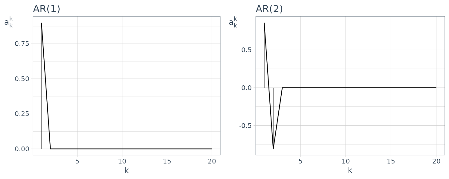
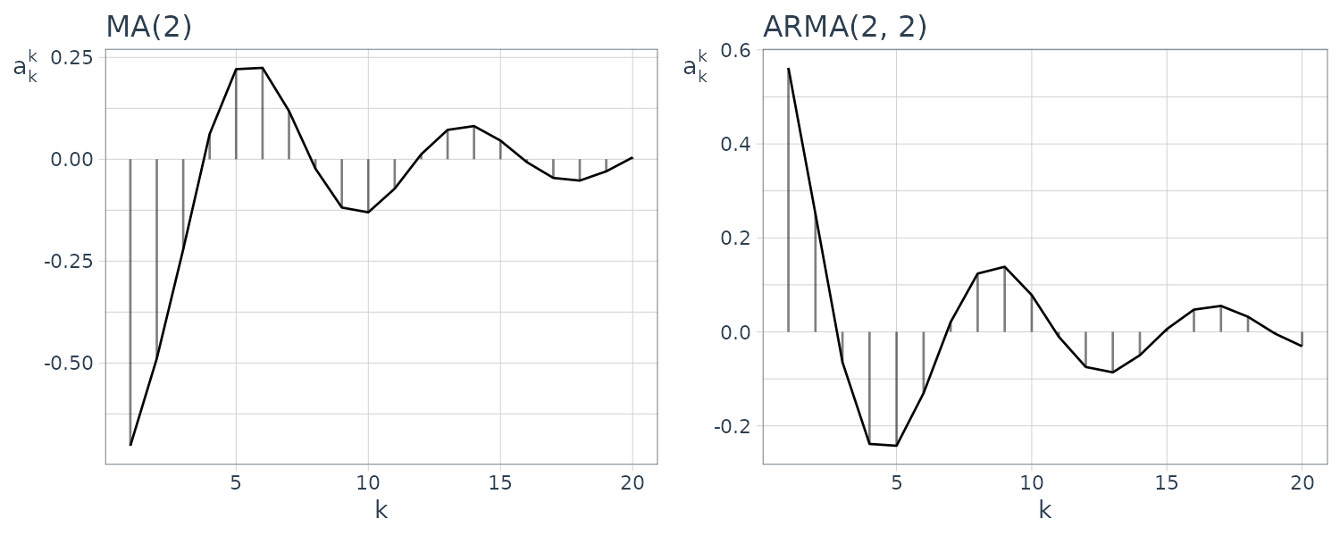
\[\begin{aligned} g_{0} &= 1 \end{aligned}\] \[\begin{aligned} g_{i} &= \sum_{j=1}^{i}a_{j}g_{i-j} - b_{i} \end{aligned}\] \[\begin{aligned} i = 1, 2, \cdots \end{aligned}\] \[\begin{aligned} a_{j} &= 0, j > m \end{aligned}\] \[\begin{aligned} b_{j} &= 0, j > l \end{aligned}\]Example: AR(1), AR(2), MA(2), and ARMA(2, 2) Models
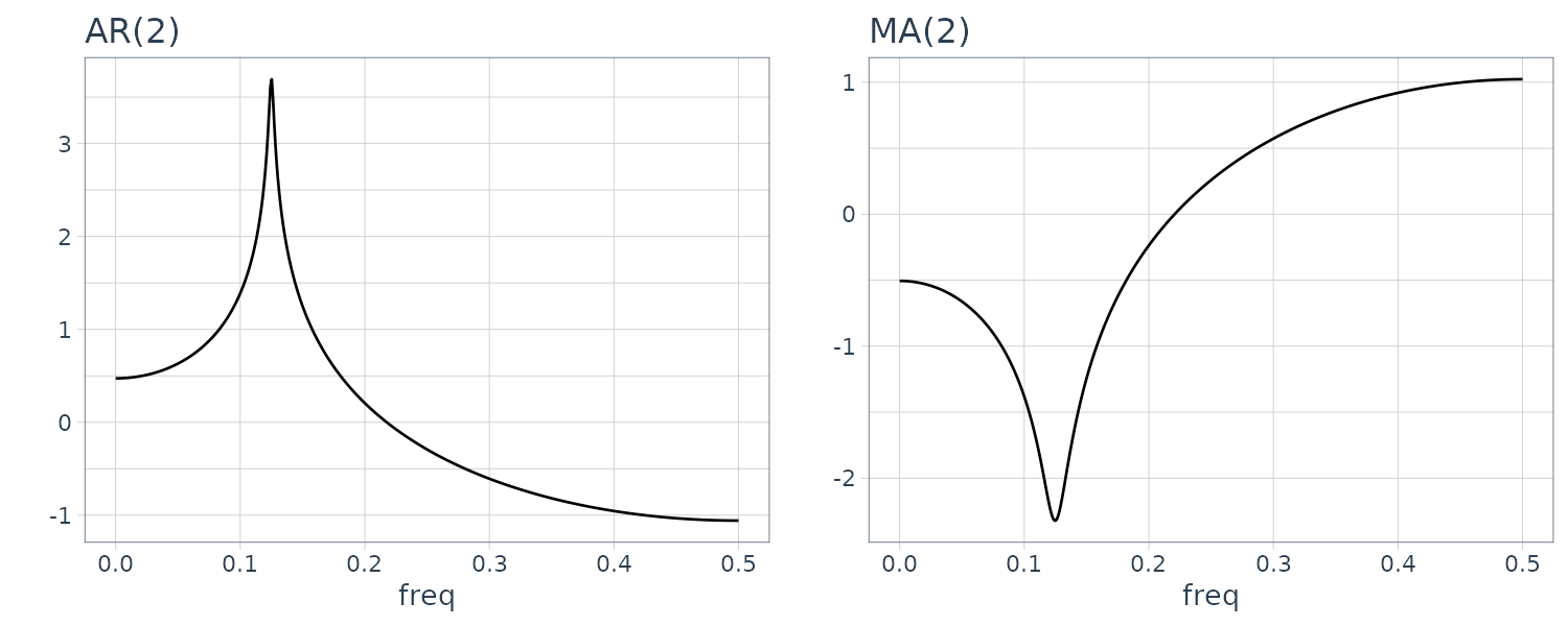
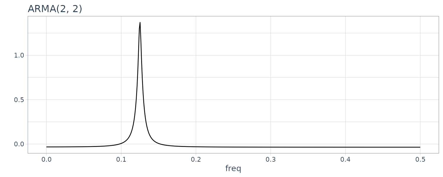
Consider the following models:
\[\begin{aligned} y_{n} &= 0.9 y_{n-1} + v_{n} \end{aligned}\] \[\begin{aligned} y_{n} &= 0.9\sqrt{3} y_{n-1} -0.81 y_{n-2} + v_{n} \end{aligned}\] \[\begin{aligned} y_{n} &= v_{n} - 0.9\sqrt{2} v_{n-1} + 0.81 v_{n-2} \end{aligned}\] \[\begin{aligned} y_{n} &= 0.9\sqrt{3} y_{n-1} -0.81 y_{n-2} + v_{n} - 0.9\sqrt{2} v_{n-1} + 0.81 v_{n-2} \end{aligned}\]The impulse response function:
dat1 <- tibble(
  g = c(
    1,
    ARMAtoMA(
      ar = 0.9,
      ma = 0,
      (n-1)
    )
  ),
  k = 1:n
)

dat2 <- tibble(
  g = c(
    1,
    ARMAtoMA(
      ar = c(0.9 * sqrt(3), -0.81),
      ma = 0,
      (n-1)
    )
  ),
  k = 1:n
)

dat3 <- tibble(
  g = c(
    1,
    ARMAtoMA(
      ar = 0,
      ma = c(-0.9 * sqrt(2), 0.81),
      (n - 1)
    )
  ),
  k = 1:n
)

dat4 <- tibble(
  g = c(
    1,
    ARMAtoMA(
      ar = c(0.9 * sqrt(3), -0.81),
      ma = c(-0.9 * sqrt(2), 0.81),
      (n - 1)
    )
  ),
  k = 1:n
)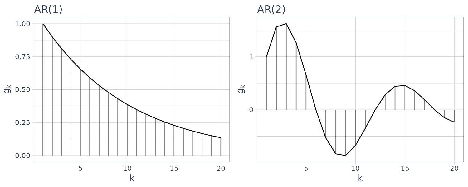
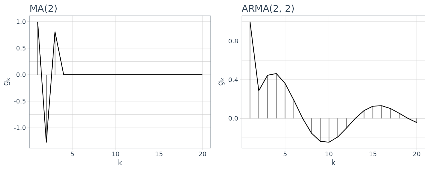
The plots above show the impulse response functions obtained from the recursive relation shown previously.
The impulse response function of the MA model is non-zero only for the initial \(l\) points. On the other hand, if the model contains an AR part, the impulse response function has non-zero values even for \(i > m\), although it gradually decays.
The Autocovariance Function
First multiply the ARMA model by \(y_{n-k}\) and take expectation:
\[\begin{aligned} y_{n} &= \sum_{i = 1}^{m}a_{i}y_{n-i} + v_{n} - \sum_{i = 1}^{l}b_{i}v_{n-i}\\ y_{n}y_{n-k} &= \sum_{i = 1}^{m}a_{i}y_{n-i}y_{n-k} + v_{n}y_{n-k} - \sum_{i = 1}^{l}b_{i}v_{n-i}y_{n-k}\\ E[y_{n}y_{n-k}] &= \sum_{i = 1}^{m}a_{i}E[y_{n-i}y_{n-k}] + E[v_{n}y_{n-k}] - \sum_{i = 1}^{l}b_{i}E[v_{n-i}y_{n-k}]\\ \end{aligned}\]Taking result from the impulse function, we can derive the covariance between the time series \(y_{m}\) and white noise \(v_{n}\):
\[\begin{aligned} E[v_{n}y_{m}] &= E[v_{n}\sum_{i=0}^{\infty}g_{i}B^{i}v_{m}]\\ &= \sum_{i=0}^{\infty}g_{i}E[v_{n}v_{m-i}]\\ &= \begin{cases} 0 & n > m\\ \sigma^{2}g_{m-n} & n \leq m \end{cases} \end{aligned}\]Since:
\[\begin{aligned} m-i &= n \end{aligned}\] \[\begin{aligned} i &= m - n \end{aligned}\]Substituting this into the above expectation, we derive the following recurrence:
\[\begin{aligned} C_{0} &= \sum_{i = 1}^{m}a_{i}E[y_{n-i}y_{n-i}] + E[v_{n}y_{n}] - \sum_{i = 1}^{l}b_{i}E[v_{n-i}y_{n}]\\ &= \sum_{i = 1}^{m}a_{i}C_{i} + \sigma^{2}g_{0} - \sum_{i = 1}^{l}b_{i}g_{n - (n - i)}\\ &= \sum_{i = 1}^{m}a_{i}C_{i} + \sigma^{2}\Big(1 - \sum_{i=1}^{l}b_{i}g_{i}\Big) \end{aligned}\] \[\begin{aligned} C_{k} &= \sum_{i = 1}^{m}a_{i}E[y_{n-i}y_{n-k}] + E[v_{n}y_{n-k}] - \sum_{i = 1}^{l}b_{i}E[v_{n-i}y_{n-k}]\\ &= \sum_{i = 1}^{m}a_{i}C_{k-i} + 0 - \sum_{i = 1}^{l}b_{i}g_{n-k - n-i}\\ &= \sum_{i = 1}^{m}a_{i}C_{k-i} - \sigma^{2}\sum_{i=1}^{l}b_{i}g_{i-k} \end{aligned}\]Therefore, if the orders m and l, the autoregressive and moving average coefficients \(a_{i}\) and \(b_{i}\), and the innovation variance \(\sigma^{2}\) of the ARMA model are given, we can obtain the autocovariance function by first computing the impulse response function \(g_{1}, \cdots, g_{l}\) and then obtaining the autocovariance function \(C_{0},C_{1}, · · ·\).
Doing this in R by using the ARMAacf() function:
n <- 20
dat1 <- tibble(
  C = ARMAacf(
    ar = 0.9,
    ma = 0,
    n
  ),
  n = 0:n
)

dat2 <- tibble(
  C = ARMAacf(
    ar = c(0.9 * sqrt(3), -0.81),
    ma = 0,
    n
  ),
  n = 0:n
)

dat3 <- tibble(
  C = ARMAacf(
    ar = 0,
    ma = c(-0.9 * sqrt(2), 0.81),
    n
  ),
  n = 0:n
)

dat4 <- tibble(
  C = ARMAacf(
    ar = c(0.9 * sqrt(3), -0.81),
    ma = c(-0.9 * sqrt(2), 0.81),
    n
  ),
  n = 0:n
)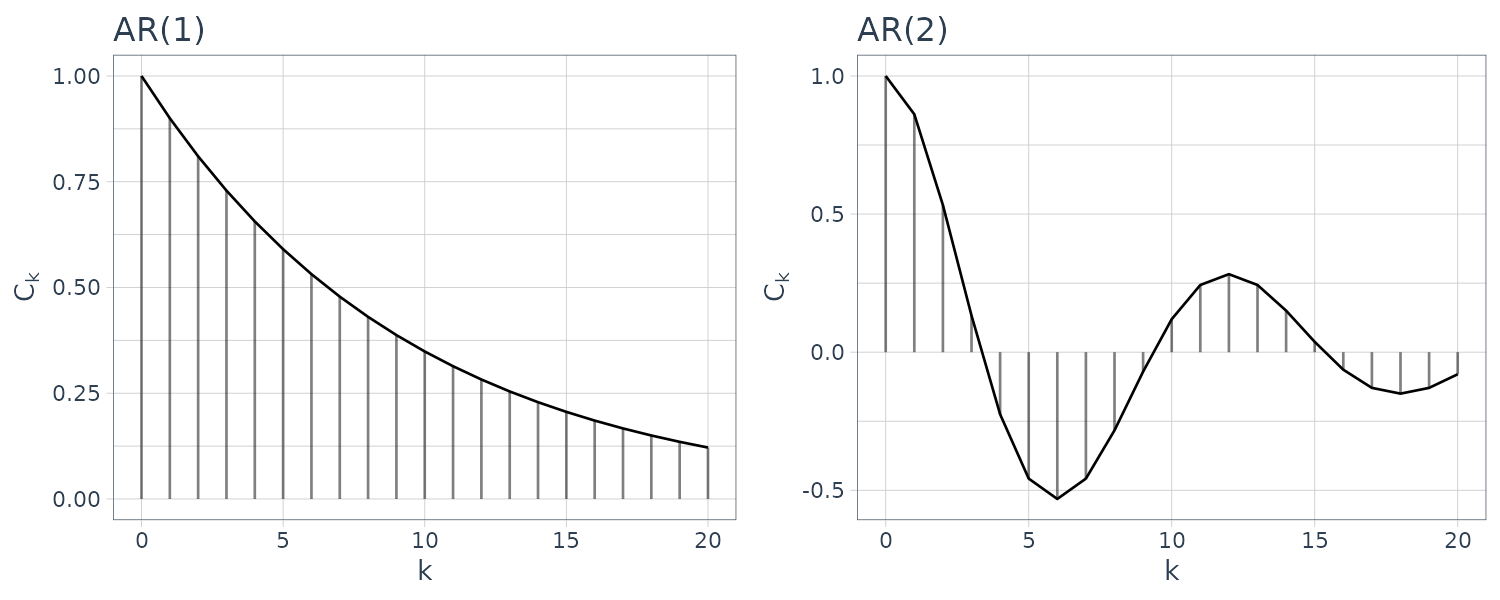
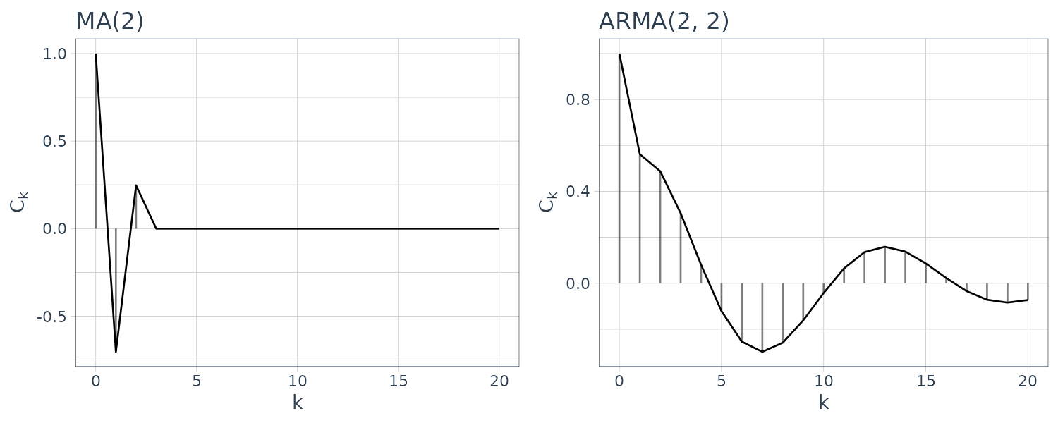
In particular, the following equation for the AR model obtained by putting \(l = 0\) is called the Yule-Walker equation:
\[\begin{aligned} C_{0} &= \sum_{i = 1}^{m}a_{i}C_{i} + \sigma^{2}\\ C_{k} &= \sum_{i = 1}^{m}a_{i}C_{k-i} \end{aligned}\]Partial Correlation
We denote the AR coefficient \(a_{i}\) of the AR model with order m as \(a_{i}^{m}\). In particular, \(a_{m}^{m}\) is called the m-th partial autocorrelation coefficient.
It can be shown the following relation holds between \(a_{i}^{m}, a_{i}^{m-1}\) (see Derivation of Levinson’s Algorithm):
\[\begin{aligned} a_{i}^{m} &= a_{i}^{m-1} - a_{m}^{m}a_{m-i}^{m-1} \end{aligned}\] \[\begin{aligned} i = 1, \cdots, m-1 \end{aligned}\]If the m PARCOR’s, \(a_{1}^{1}, \cdots, a_{m}^{m}\), are given, repeated application of above equation yields the entire set of coefficients of the AR models with orders 2 through m.
On the other hand, if the coefficients \(a_{1}^{m}, \cdots, a_{m}^{m}\) of the AR model of the highest order are given and by solving the following equations:
\[\begin{aligned} a_{i}^{m-1} &= \frac{a_{i}^{m} + a_{m}^{m}a_{m-i}^{m}}{1 - (a_{m}^{m})^{2}} \end{aligned}\]The coefficients of the AR model with order \(m-1\) are obtained.
To show this, given:
\[\begin{aligned} a_{i}^{m} &= a_{i}^{m-1} - a_{m}^{m}a_{m-i}^{m-1} \end{aligned}\]And substituting \(i\) with \(m-i\):
\[\begin{aligned} a_{m-i}^{m} &= a_{i}^{m-1} - a_{m}^{m}a_{m-(m-i)}^{m-1}\\ a_{i}^{m-1} &= a_{m-i}^{m} + a_{m}^{m}a_{i}^{m-1} \end{aligned}\]Substituting \(a_{i}^{m-1}\):
\[\begin{aligned} a_{i}^{m} &= a_{i}^{m-1}- a_{m}^{m}(a_{m-i}^{m} + a_{m}^{m}a_{i}^{m-1})\\ &= a_{i}^{m-1}- a_{m}^{m}a_{m-i}^{m} - (a_{m}^{m})^{2}a_{i}^{m-1}\\ &= a_{i}^{m-1}(1 - a_{m}^{m}) - (a_{m}^{m})^{2}a_{m-i}^{m} \end{aligned}\] \[\begin{aligned} a_{i}^{m-1} &= \frac{a_{i}^{m} + a_{m}^{m}a_{m-i}^{m}}{1 - (a_{m}^{m})^{2}} \end{aligned}\]The PARCORs, \(a_{1}^{1}, \cdots, a_{m}^{m}\), can be obtained by repeating the above computation.
This reveals that estimation of the coefficients \(a_{1}^{m}, \cdots, a_{m}^{m}\) of the AR model of order m is equivalent to estimation of the PARCOR’s up to the order m, i.e., \(a_{1}^{1}, \cdots, a_{m}^{m}\).
The following R code shows the PARCOR of the four models by using the same ARMAacf() function but having the argument pacf = TRUE:
dat1 <- tibble(
  C = ARMAacf(
    ar = 0.9,
    ma = 0,
    n,
    pacf = TRUE
  ),
  n = 1:n
)

dat2 <- tibble(
  C = ARMAacf(
    ar = c(0.9 * sqrt(3), -0.81),
    ma = 0,
    n,
    pacf = TRUE
  ),
  n = 1:n
)

dat3 <- tibble(
  C = ARMAacf(
    ar = 0,
    ma = c(-0.9 * sqrt(2), 0.81),
    n,
    pacf = TRUE
  ),
  n = 1:n
)

dat4 <- tibble(
  C = ARMAacf(
    ar = c(0.9 * sqrt(3), -0.81),
    ma = c(-0.9 * sqrt(2), 0.81),
    n,
    pacf = TRUE
  ),
  n = 1:n
)
The Power Spectrum of the ARMA Process
Recall the power spectrum is defined as:
\[\begin{aligned} p(f) &= \sum_{k=-\infty}^{\infty}C_{k}e^{-2\pi i k f} \end{aligned}\]If an ARMA model of a time series is given, the power spectrum of the time series can be obtained easily:
\[\begin{aligned} p(f) &= \sum_{k=-\infty}^{\infty}C_{k}e^{-2\pi i k f}\\ &= \sum_{k=-\infty}^{\infty}E[y_{n}y_{n-k}]e^{-2\pi i k f}\\ &= \sum_{k=-\infty}^{\infty}E\Big[\sum_{j=0}^{\infty}g_{j}v_{n-j}\sum_{p=0}^{\infty}g_{p}v_{n-k-p}\Big]e^{-2\pi i k f}\\ &= \sum_{k=-\infty}^{\infty}\sum_{j=0}^{\infty}\sum_{p=0}^{\infty}g_{j}g_{p}E[v_{n-j}v_{n-k-p}]e^{-2\pi i k f} \end{aligned}\]Here using \(g_{p} = 0\) for \(p < 0\) and:
\[\begin{aligned} n - k - p &= n - j\\ p &= n - k - (n - j)\\ &= j - k \end{aligned}\]The power spectrum is expressed as:
\[\begin{aligned} p(f) &= \sigma^{2}\sum_{k=-\infty}^{\infty}\sum_{j=0}^{\infty}g_{j}g_{n - k - (j-k)}e^{-2\pi i k f}\\ &= \sigma^{2}\sum_{k=-\infty}^{\infty}\sum_{j=0}^{\infty}g_{j}g_{j-k}e^{-2\pi i k f}\\ &= \sigma^{2}\sum_{k=-\infty}^{\infty}\sum_{j=0}^{\infty}g_{j}g_{j-k}e^{-2\pi i j f +2 \pi ijf - 2\pi ikf}\\ &= \sigma^{2}\sum_{k=-\infty}^{\infty}\sum_{j=0}^{\infty}g_{j}g_{j-k}e^{-2\pi ijf - 2\pi(k-j)f}\\ &= \sigma^{2}\sum_{k=-\infty}^{\infty}\sum_{j=0}^{\infty}g_{j}e^{-2\pi i j f}g_{j-k}e^{-2\pi i (k-j) f}\\ &= \sigma^{2}\sum_{j=0}^{\infty}\sum_{p=0}^{\infty}g_{j}e^{-2\pi i j f}g_{p}e^{2\pi i p f}\\ &= \sigma^{2}\Big|\sum_{j=0}^{\infty}g_{j}e^{-2\pi i j f}\Big|^{2} \end{aligned}\]\(\sum_{j=0}^{\infty}g_{j}e^{-2\pi i j f}\) is the Fourier transform of the impulse response function, and is called the frequency response function.
Focusing on the frequency response function:
\[\begin{aligned} \sum_{j=0}^{\infty}g_{j}e^{-2\pi i j f} &= \frac{1 - \sum_{j=1}^{l}b_{j}e^{-2\pi ijf}}{1 - \sum_{j=1}^{m}a_{j}e^{-2\pi i j f}} \end{aligned}\]Therefore the power spectrum can be derived from the ARMA model by:
\[\begin{aligned} p(f) &= \sigma^{2}\frac{\Big|1 - \sum_{j=1}^{l}b_{j}e^{-2\pi ijf}\Big|^{2}}{\Big|1 - \sum_{j=1}^{m}a_{j}e^{-2\pi i j f}\Big|^{2}} \end{aligned}\]Example
Computing the log-spectrum for the 4 models:
sp1 <- astsa::arma.spec(0.9)

sp2 <- astsa::arma.spec(
  ar = c(0.9 * sqrt(3), -0.81)
)

sp3 <- astsa::arma.spec(
  ma = c(-0.9 * sqrt(2), 0.81)
)

sp4 <- astsa::arma.spec(
  ar = c(0.9 * sqrt(3), -0.81),
  ma = c(-0.9 * sqrt(2), 0.81)
)

tibble(
  freq = sp1$freq,
  spec = log10(sp1$spec)
) |>
  ggplot(aes(x = freq, y = spec)) +
  geom_line() +
  ggtitle("AR(1)") +
  theme_tq()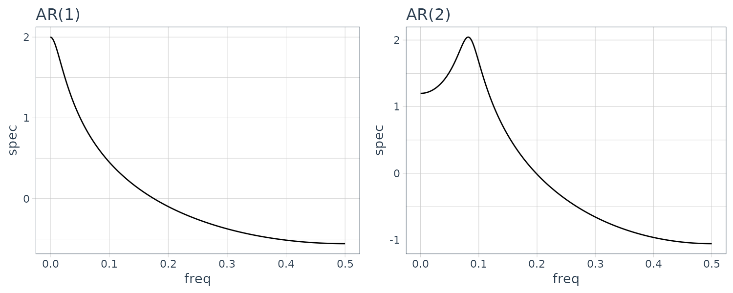
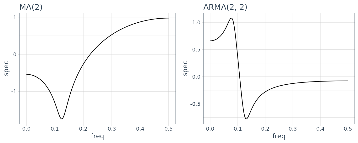
The power spectrum of the AR model with order 1 does not have any peak or trough. A peak is seen in the spectrum of the 2nd order AR model and one trough is seen in the plot of the 2nd order MA model. On the other hand, the spectrum of the ARMA model of order (2,2) shown in the plot has both one peak and one trough.
The logarithm of the spectrum is expressible as:
\[\begin{aligned} \log p(f) &= \log \sigma^{2} - 2 \log\Big|1 - \sum_{j=1}^{m}a_{j}e^{-2\pi ijf}\Big| + 2 \log\Big|1 - \sum_{j=1}^{l}b_{j}e^{-2\pi ijf}\Big| \end{aligned}\]Therefore, the peak and the trough of the spectrum appear at the local minimum of \(\mid 1 - \sum_{j=1}^{m}a_{j}e^{-2\pi ijf}\mid\) and \(\mid 1 - \sum_{j=1}^{l}b_{j}e^{-2\pi ijf}\mid\), respectively.
To express k peaks or k troughs, the AR order or the MA order must be higher than or equal to 2k, respectively. Moreover, the locations and the heights of the peaks or the troughs are related to the angles and the absolute values of the complex roots of the characteristic equation.
The Characteristic Equation
The characteristics of an ARMA model are determined by the roots of the following two polynomial equations:
\[\begin{aligned} a(B) &= 1 - \sum_{j=1}^{m}a_{j}B^{j} = 0\\ b(B) &= 1 - \sum_{j=1}^{l}b_{j}B^{j} = 0 \end{aligned}\]The roots of these equations are called the characteristic roots. If the roots of the characteristic equation \(a(B) = 0\) of the AR operator all lie outside the unit circle, the influence of noise turbulence at a certain time decays as time progresses, and the ARMA model becomes stationary.
On the other hand, if all roots of the characteristic equation \(b(B) = 0\) of the MA operator lie outside the unit circle, the coefficient of \(h_{i}\) of \(b(B)^{−1} = \sum_{i=0}^{\infty}h_{i}B^{i}\) converges and the ARMA model can be expressed by an AR model of infinite order as:
\[\begin{aligned} y_{n} &= -\sum_{i=1}^{\infty}h_{i}y_{n-i} + v_{n} \end{aligned}\]In this case, the time series is called invertible.
In particular, when the angles of the complex roots of the AR operator coincide with those of the MA operator, a line-like spectral peak or trough appears.
For example, if the AR and MA coefficients of the ARMA (2,2) model are given by:
\[\begin{aligned} a_{1} &= 0.99\sqrt{2}\\ a_{2} &= -0.99^{2}\\ b_{1} &= 0.95\sqrt{2}\\ b_{2} &= -0.95^{2} \end{aligned}\]Both characteristic equations have roots at \(f = 0.125\) (\(0.125 \times 460 = 45\)):
> polyroot(c(1, -0.99 * sqrt(2), 0.99^2)) |>
  Arg() * 180 / pi
[1]  45 -45

> polyroot(c(1, -0.95 * sqrt(2), 0.95^2)) |>
  Arg() * 180 / pi
[1]  45 -45
And the spectral:
sp1 <- astsa::arma.spec(
  ar = c(0.99 * sqrt(2), -0.99^2)
)

sp2 <- astsa::arma.spec(
  ma = c(-0.95 * sqrt(2), 0.95^2)
)

sp3 <- astsa::arma.spec(
  ar = c(0.99 * sqrt(2), -0.99^2),
  ma = c(-0.95 * sqrt(2), 0.95^2)
)
The peak of the spectrum (or trough) appears at \(f = \frac{\theta}{2\pi}\), if the complex root of AR (or MA) operator is expressed in the form:
\[\begin{aligned} z &= \alpha + i\beta\\ &= re^{i\theta} \end{aligned}\]Further, the closer the root r approaches to 1, the sharper the peak or the trough of the spectrum become.
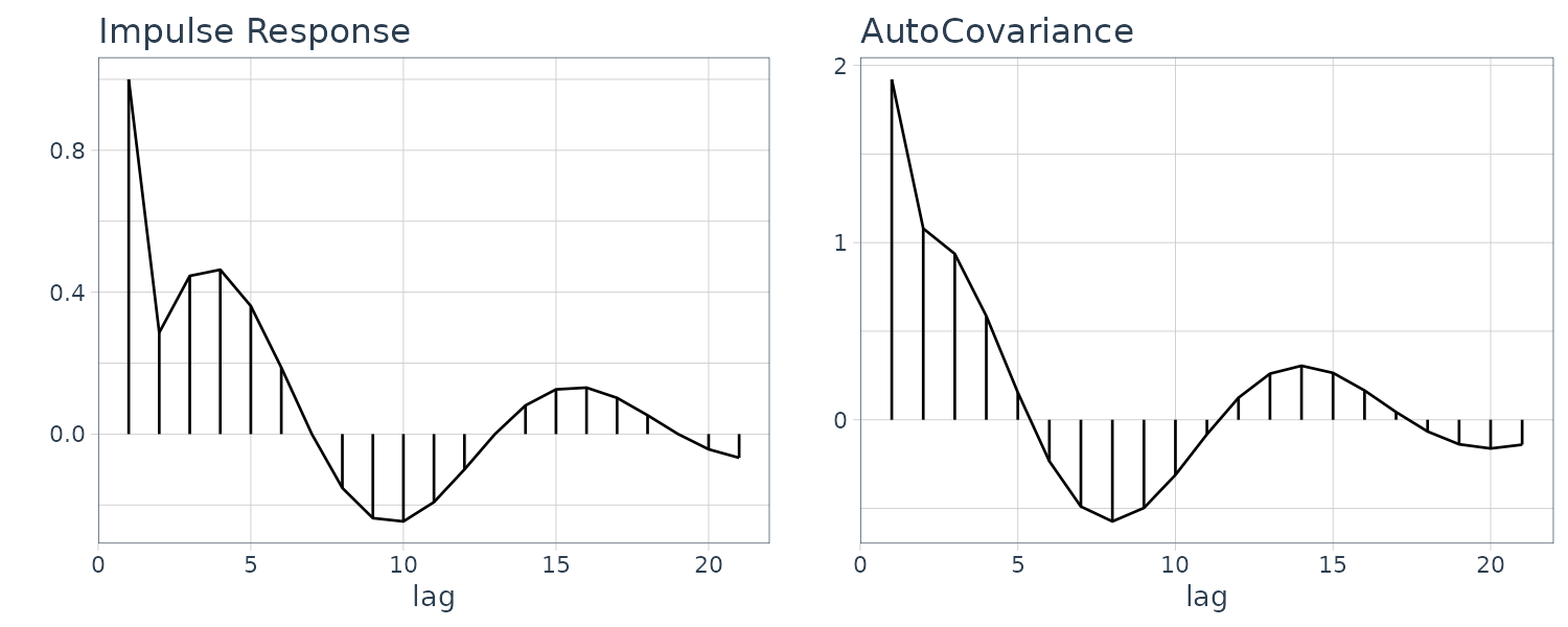
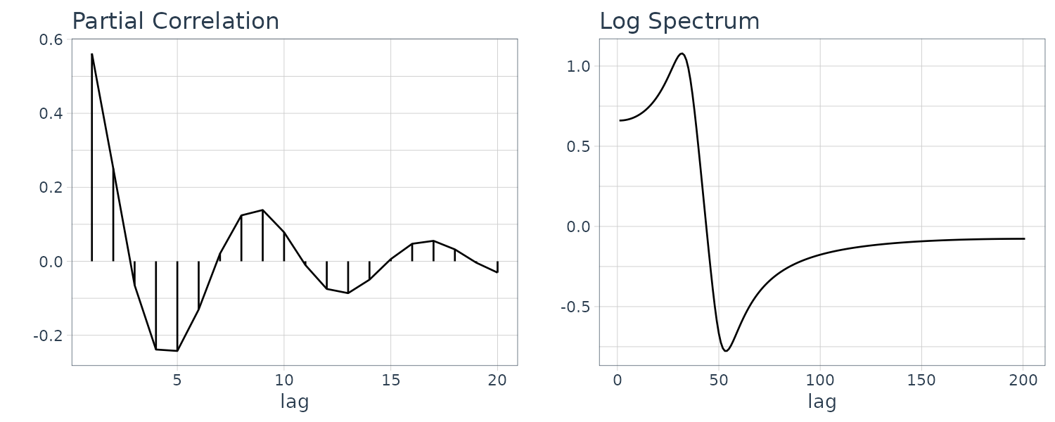
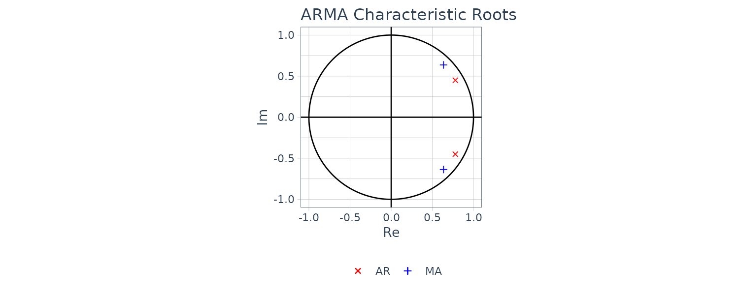
The function armachar of the package TSSS computes and draw graphs of the impulse response function, the autocovariance function, the PARCORs, power spectrum and the characteristic roots of the AR operator and the MA operator of an ARMA model.
For example the following AR, MA, and ARMA models:
\[\begin{aligned} y_{n} &= 0.9\times \sqrt{3}y_{n-1} - 0.81y_{n-2} + v_{n}\\ y_{n} &= v_{n} - 0.9\times \sqrt{2} + 0.81v_{n-2} \end{aligned}\] \[\begin{aligned} y_{n} &= 0.9\times \sqrt{3}y_{n-1} - 0.81y_{n-2} + v_{n} - 0.9\times \sqrt{2} + 0.81v_{n-2} \end{aligned}\]a <- c(0.99 * sqrt(2), -0.9801)
b <- c(0.95 * sqrt(2), -0.9025)
fit <- armachar(
arcoef = a,
macoef = b,
v = 1.0,
lag = 20
)
> names(fit)
[1] "impuls" "acov" "parcor" "spec"
[5] "croot.ar" "croot.ma"Note that the inverse roots are graphed instead so the points are inside rather than outside the unit circle.
The Multivariate AR Model
Similar to the case of univariate time series, for multivariate time series:
\[\begin{aligned} \textbf{y}_{n} &= \begin{bmatrix} y_{n}(1)\\ \vdots\\ y_{n}(l) \end{bmatrix} \end{aligned}\]The model that expresses a present value of the time series as a linear combination of past values \(\textbf{y}_{n−1}, \cdots, \textbf{y}_{n−M}\) and white noise is called a multivariate autoregressive model (MAR model):
\[\begin{aligned} \textbf{y}_{n} &= \sum_{m=1}^{M}\textbf{A}_{m}\textbf{y}_{n-m} + \textbf{v} \end{aligned}\]Where \(\textbf{A}_{m}\) is the autoregressive coefficient matrix whose (i, j)-th element is given by \(a_{m}(i, j)\), and \(v_{n}\) is an l-dimensional white noise that satisfies:
\[\begin{aligned} E[\textbf{v}_{n}] &= \begin{bmatrix} 0\\ \vdots\\ 0 \end{bmatrix} \end{aligned}\] \[\begin{aligned} E[\textbf{v}_{n}\textbf{v}_{n}^{T}] &= \begin{bmatrix} \sigma_{11} & \cdots & \sigma_{1l}\\ \vdots & \ddots & \vdots\\ \sigma_{l1} & \cdots & \sigma_{ll} \end{bmatrix} = \textbf{W} \end{aligned}\] \[\begin{aligned} E[\textbf{v}_{n}\textbf{v}_{m}^{T}] &= \textbf{0}_{n \times m}, n \neq m \end{aligned}\] \[\begin{aligned} E[\textbf{v}_{n}\textbf{y}_{m}^{T}] &= \textbf{0}_{n\times m}, n > m \end{aligned}\]The cross-covariance function of \(\textbf{y}_{n}(i), \textbf{y}_{n}(j)\) is defined by:
\[\begin{aligned} \textbf{C}_{k}(i, j)&= E[\textbf{y}_{n}(i)\textbf{y}_{n-k}(j)] \end{aligned}\]For the \(l \times l\) matrix:
\[\begin{aligned} \textbf{C}_{k} = E[\textbf{y}_{n}\textbf{y}_{n-k}^{T}] \end{aligned}\]The (i, j)-th component of which is \(\textbf{C}_{k}(i, j)\), is called the cross-covariance function.
Similar to the case of the univariate time series, for the multivariate AR model, \(\textbf{C}_{k}\) satisfies the Yule-Walker equation:
\[\begin{aligned} \textbf{C}_{0} &= \sum_{j=1}^{M}\textbf{A}_{j}\textbf{C}_{-j} + \textbf{W}\\ \textbf{C}_{k} &= \sum_{j=1}^{M}\textbf{A}_{j}\textbf{C}_{k-j} \end{aligned}\] \[\begin{aligned} k = 1, 2, \cdots \end{aligned}\]The cross-covariance function is not symmetric. Therefore, for multivariate time series, the Yule-Walker equations for the the backward AR model and the forward AR model are different.
The Fourier transform of the cross-covariance function \(\textbf{C}_{k}(s, j)\) is called the cross-spectral density function:
\[\begin{aligned} p_{sj}(f) &= \sum_{k=-\infty}^{\infty}\textbf{C}_{k}(s, j)e^{-2\pi i k f}\\ &= \sum_{k=-\infty}^{\infty}\textbf{C}_{k}(s, j)\textrm{cos}(2\pi k f) - i\sum_{k=-\infty}^{\infty}\textbf{C}_{k}(s, j)\textrm{sin}(2\pi k f) \end{aligned}\]Since the cross-covariance function is not an even function, the cross-spectrum given by:
\[\begin{aligned} \textbf{P}(f) &= \begin{bmatrix} p_{11}(f) & \cdots & p_{1l}(f)\\ \vdots & \ddots & \vdots\\ p_{l1}(f) & \cdots & p_{ll}(f) \end{bmatrix} \end{aligned}\]And has an imaginary part and is a complex number.
And the relations between \(\mathbf{P}(f)\) and the cross-covariance matrix \(\textbf{C}_{k}\) are given by:
\[\begin{aligned} \mathbf{P}(f) &= \sum_{k=-\infty}^{\infty}\textbf{C}_{k}e^{-2\pi i k f}\\ \textbf{C}_{k} &= \int_{-\frac{1}{2}}^{\frac{1}{2}}\mathbf{P}(f)e^{2\pi i k f}\ df \end{aligned}\]For time series that follow the multivariate AR model, the cross-spectrum can be obtained by:
\[\begin{aligned} \mathbf{P}(f) &= \textbf{A}(f)^{-1}\textbf{W}(\textbf{A}(f)^{-1})^{*} \end{aligned}\]Where \(\textbf{A}^{*}\) denotes the complex conjugate of the matrix \(\textbf{A}\), and \(\textbf{A}(f)\) denotes the \(l \times l\) matrix whose (j, k)-th component is defined by:
\[\begin{aligned} \textbf{A}_{jk}(f) &= \sum_{m=0}^{M}a_{m}(j, k)e^{-2\pi i m f} \end{aligned}\]Here, it is assumed that:
\[\begin{aligned} a_{0}(j, j) &= −1 \end{aligned}\] \[\begin{aligned} a_{0}(j, k) &= 0, j \neq k \end{aligned}\]Given a frequency f, the cross-spectrum is a complex number and can be expressed as:
\[\begin{aligned} p_{jk}(f) &= \alpha_{jk}(f)e^{i\phi_{jk}(f)} \end{aligned}\]Where:
\[\begin{aligned} \alpha_{jk}(f) &= \sqrt{\mathrm{Re}(p_{jk}(f))^{2} + \mathrm{Im}(p_{jk}(f))^{2}}\\ \phi_{jk}(f) &= \mathrm{arctan}\Bigg(\frac{\mathrm{Im}(p_{jk}(f))}{\textrm{Re}(p_{jk}(f))}\Bigg) \end{aligned}\]\(\alpha_{jk}(f)\) is called the amplitude spectrum and \(\phi_{jk}(f)\) is the phase spectrum.
The following denotes the the square of the correlation coefficient between frequency components of time series \(\textbf{y}_{n}(j)\) and \(\textbf{y}_{n}(k)\) at frequency f and is called the coherency:
\[\begin{aligned} \textrm{coh}_{jk}(f) &= \frac{\alpha_{jk}(f)^{2}}{p_{jj}(f)p_{kk}(f)} \end{aligned}\]For convenience, in the following \(\textbf{A}(f)^{-1}\) will be denoted as \(\textbf{B}(f) = \{b_{jk}(f)\}\).
If the components of the white noise \(\textbf{v}_{n}\) are mutually uncorrelated and the variance covariance matrix is the diagonal matrix:
\[\begin{aligned} \textbf{W} &= \begin{bmatrix} \sigma_{1}^{2} & &\\ & \ddots &\\ &&\sigma_{l}^{2} \end{bmatrix} \end{aligned}\]Then the power spectrum of the i-th component of the time series can be expressed as:
\[\begin{aligned} p_{ii}(f) &= \sum_{j=1}^{l}b_{ij}(f)\sigma_{j}^{2}b_{ij}(f)^{*}\\ &= \sum_{j=1}^{l}|b_{ij}(f)|^{2}\sigma_{j}^{2} \end{aligned}\]This indicates that the power of the fluctuation of the component i at frequency \(f\) can be decomposed into the effects of \(l\) noises.
Therefore, if we define \(r_{ij}(f)\) by:
\[\begin{aligned} r_{ij}(f) &= \frac{|b_{ij}(f)|^{2}\sigma_{j}^{2}}{p_{ii}(f)} \end{aligned}\]It represents the ratio of the effect of \(\textbf{v}_{n}(j)\) in the fluctuation of \(\textbf{y}_{n}(i)\) at frequency f. This quantity \(r_{ij}(f)\) is called the relative power contribution.
Example:
The function marspc of the package TSSS computes the cross-spectra, the coherency and the power contribution of multivariate time series.
The following arguments are required:
- arcoef: AR coefficient matrices.
- v: innovation covariance matrix.
And the outputs from this function are:
- spec: cross-spectra.
- amp: amplitude spectra.
- phase: phase spectra.
- coh: simple coherency.
- power: power contribution.
- rpower: relative power contribution.
Using the HAKUSAN dataset:
\[\begin{aligned} \textbf{y}_{n} &= \begin{bmatrix} y_{n}(\text{Yaw})\\ y_{n}(\text{Pitch})\\ y_{n}(\text{Rudder}) \end{bmatrix} \end{aligned}\]We take half (N = 500) of the samples at \(\Delta t = 2\):
yy <- HAKUSAN |>
  spread(key = key, value = value) |>
  as_tibble() |>
  select(YawRate, Rolling, Rudder) |>
  as.matrix()

nc <- dim(yy)[1]
n <- seq(1, nc, by = 2)
y <- yy[n, ]

# Fit MAR model
fit <- marfit(y, lag = 20)

> fit

 Order     AIC
    0      7091.707
    1      6238.803
    2      5275.361
    3      5173.022
    4      5135.199
    5      5136.631
    6      5121.019
    7      5105.826
    8      5096.349
    9      5087.905
   10      5093.793
   11      5091.420
   12      5099.441
   13      5097.981
   14      5100.978
   15      5113.050
   16      5116.516
   17      5129.417
   18      5136.063
   19      5143.562
   20      5157.365

 Minimum AIC = 5087.905  attained at m = 9

 Innovation covariance matrix
  2.225414e+00 -4.712800e-01 -3.402811e-01
 -4.712800e-01  7.129234e-01  1.063104e-01
 -3.402811e-01  1.063104e-01  2.781570e+00

> names(fit)
[1] "maice.order" "aic" "v" "arcoef"
To retrieve the spectral, coherence and power calculations:
fit <- marspc(
  fit$arcoef,
  v = fit$v,
  plot = FALSE
)

> names(fit)
[1] "spec"   "amp"    "phase"  "coh"    "power"  "rpower"
The power spectral for the 3 series:
n <- 200
dat <- tibble(
  yaw_spec = fit$spec[, 1, 1],
  pitch_spec = fit$spec[, 2, 2],
  rudder_spec = fit$spec[, 3, 3],
  x = seq(0, 0.5, length.out = n + 1)
)

dat |>
  ggplot(
    aes(
      x = x,
      y = log10(Mod(yaw_spec))
    )
  ) +
  geom_line() +
  xlab("Freq") +
  ylab("Log-Power") +
  ggtitle("Yaw") +
  theme_tq()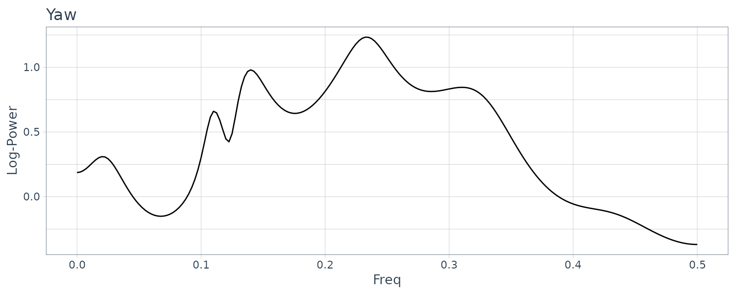
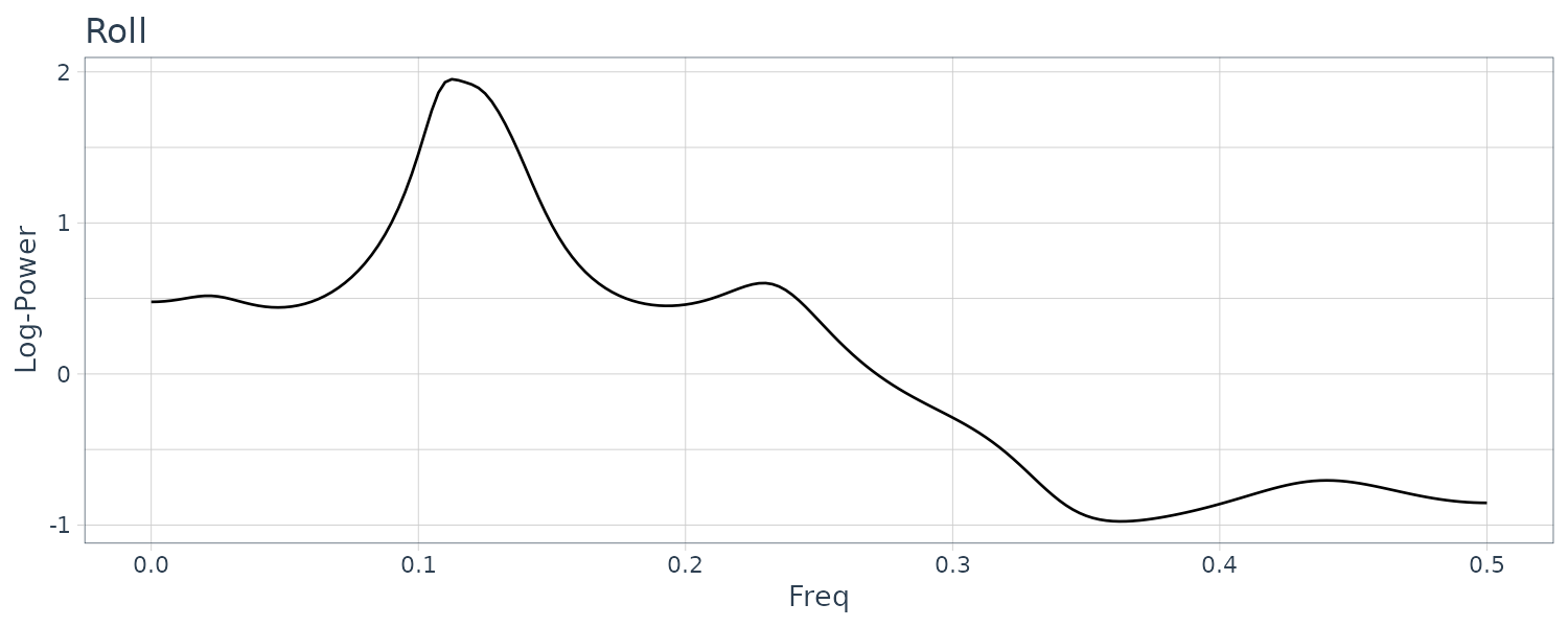

For the power spectra of the yaw rate, the maximum peak is seen in the vicinity of \(f = 0.25\) (8 seconds cycle) and for the role rate and the rudder angle in the vicinity of \(f = 0.125\) (16 seconds cycle).
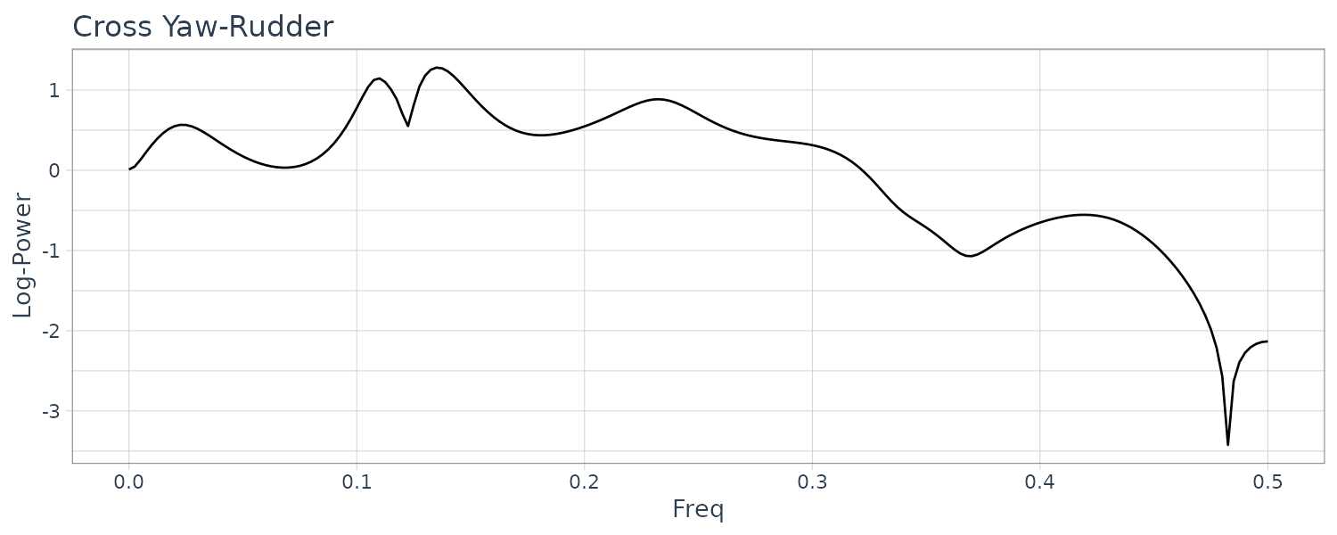
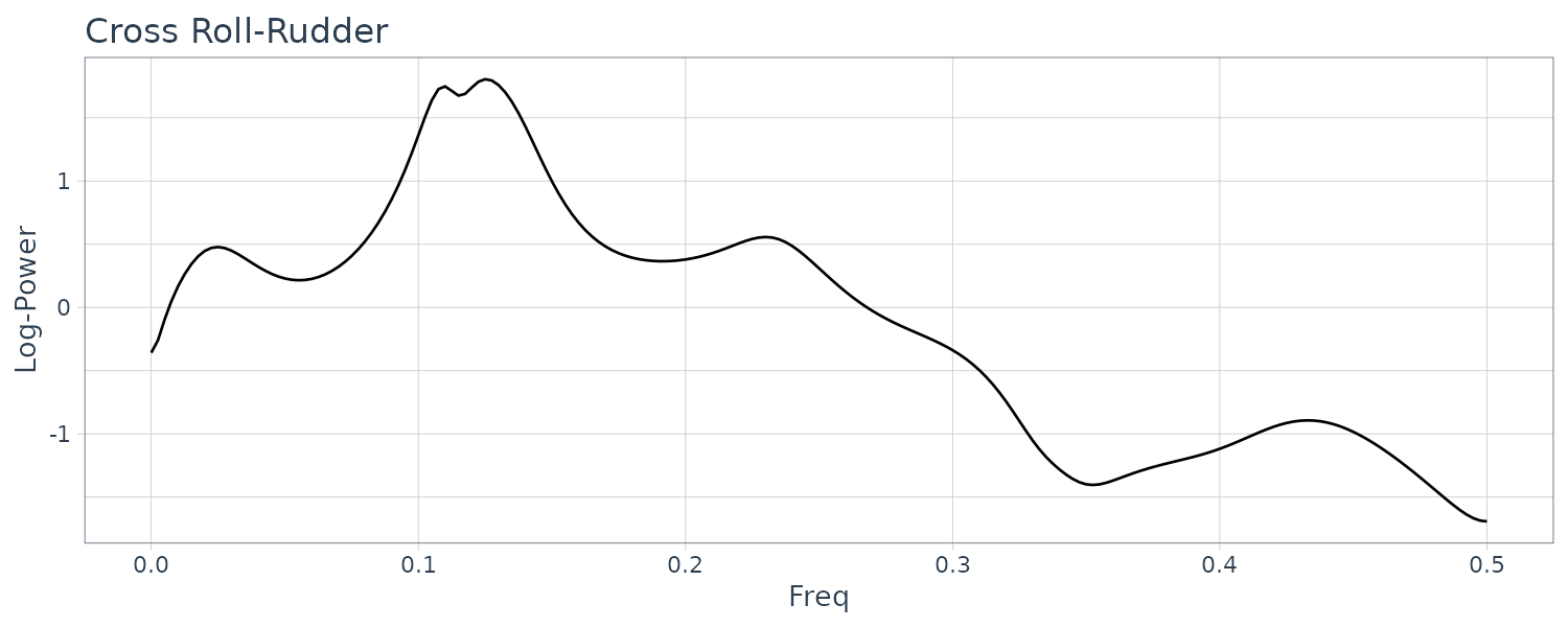
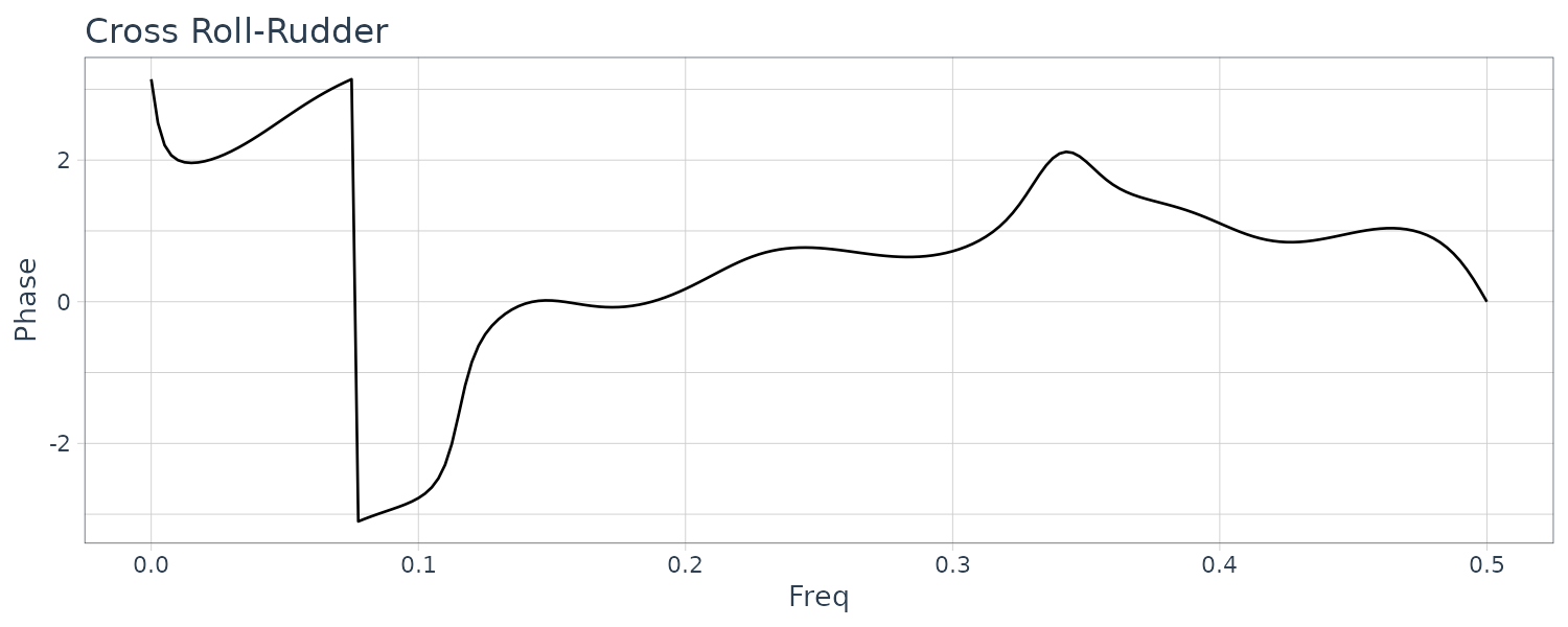
Cross Phase Spectral:
dat <- tibble(
  yaw_pitch = fit$spec[, 1, 2],
  yaw_rudder = fit$spec[, 1, 3],
  pitch_rudder = fit$spec[, 2, 3],
  x = seq(0, 0.5, length.out = n + 1)
)

dat |>
  ggplot(aes(x = x, y = log10(Mod(yaw_pitch)))) +
  geom_line() +
  xlab("Freq") +
  ylab("Log-Power") +
  ggtitle("Cross Yaw-Pitch") +
  theme_tq()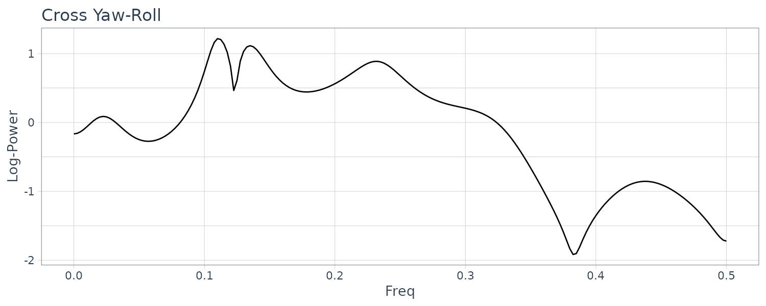
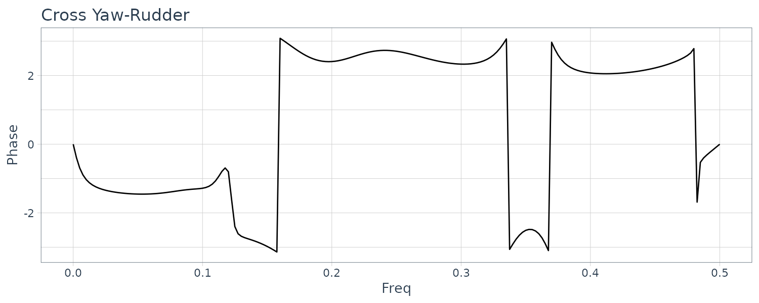
Note that phase spectra below are displayed within the range \([-\pi, \pi]\):
dat |>
  ggplot(aes(x = x, y = Arg(yaw_pitch))) +
  geom_line() +
  xlab("Freq") +
  ylab("Phase") +
  ggtitle("Cross Yaw-Pitch") +
  theme_tq()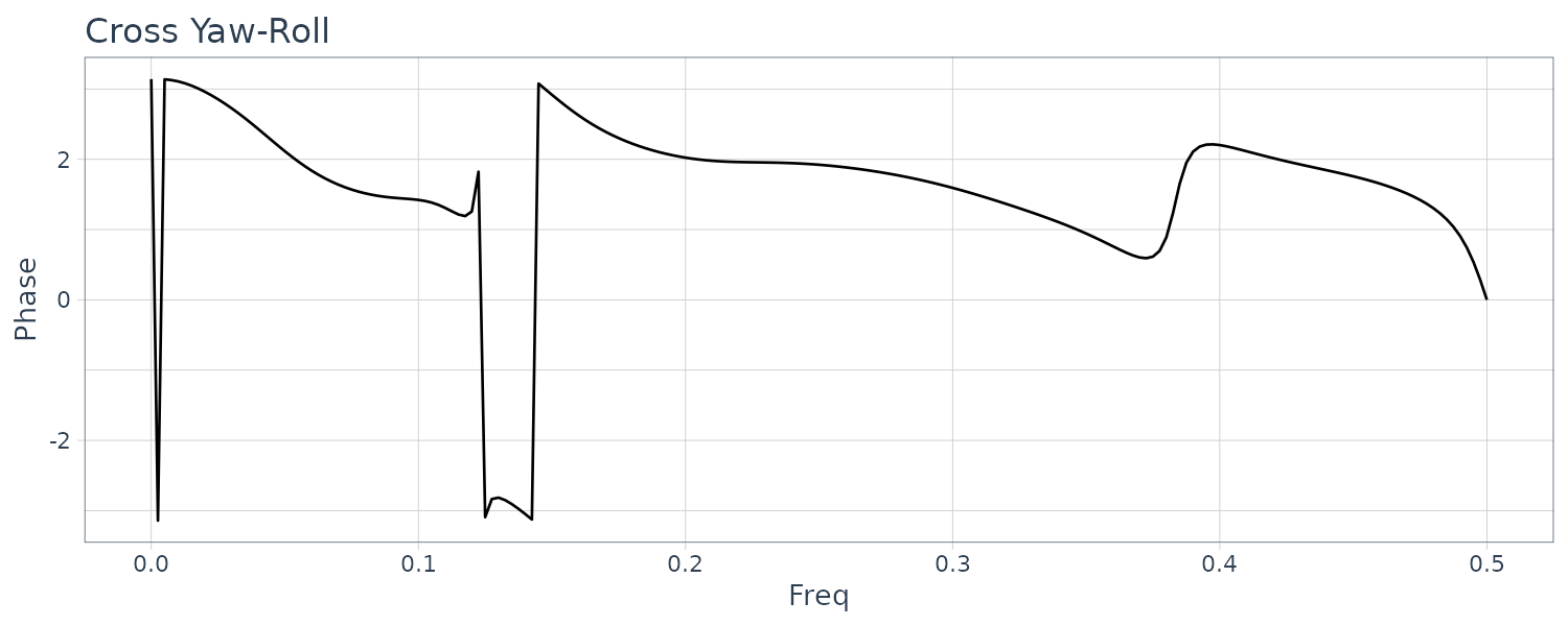
Coherencies:
dat <- tibble(
  yaw_pitch = fit$coh[, 1, 2],
  yaw_rudder = fit$coh[, 1, 3],
  pitch_rudder = fit$coh[, 2, 3],
  x = seq(0, 0.5, length.out = n + 1)
)

dat |>
  ggplot(
    aes(
      x = x,
      y = yaw_pitch
    )
  ) +
  geom_line() +
  xlab("Freq") +
  ylab("Coherency") +
  ggtitle("Coherency Yaw-Pitch") +
  theme_tq()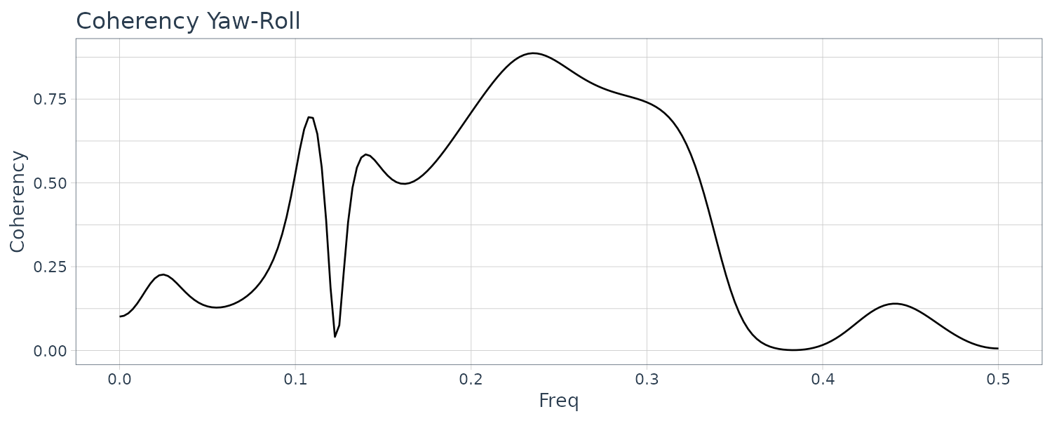
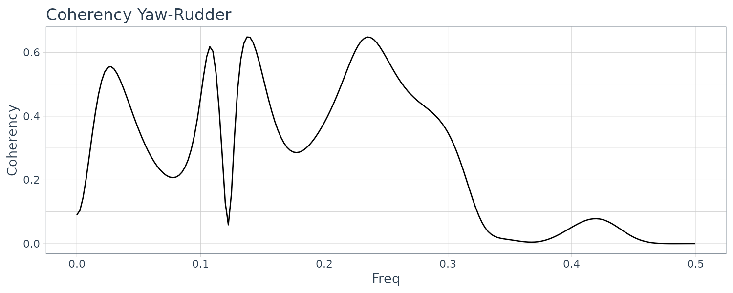
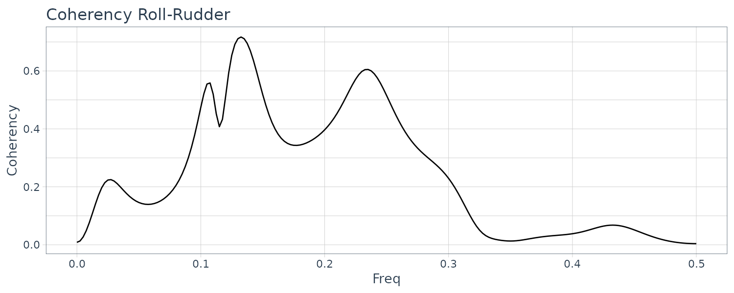
Yaw and rudder angle have two significant peaks at the same frequencies. The peak of the yaw rate has slightly smaller frequency than those of yaw rate and rolling.
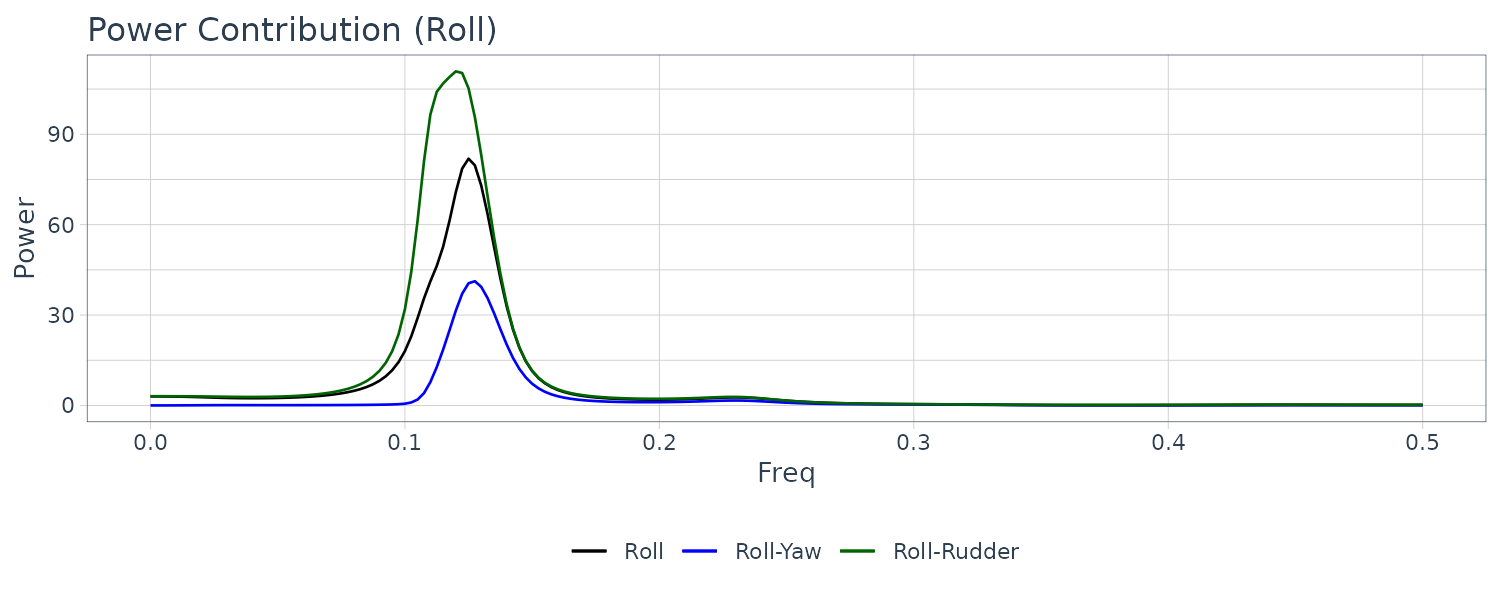
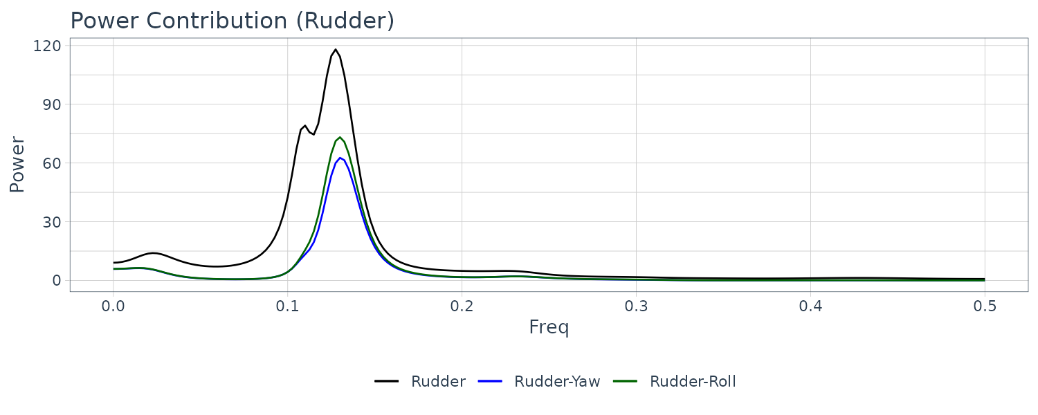
Power Contributions in terms of the \(l\) noises \(\mid b_{ij}(f)\mid^{2}\):
dat <- tibble(
  yaw = fit$power[, 1, 1],
  yaw_pitch = fit$power[, 1, 2],
  yaw_rudder = fit$power[, 1, 3],
  pitch = fit$power[, 2, 2],
  pitch_yaw = fit$power[, 2, 1],
  pitch_rudder = fit$power[, 2, 3],
  rudder = fit$power[, 3, 3],
  rudder_yaw = fit$power[, 3, 1],
  rudder_pitch = fit$power[, 3, 2],
  x = seq(0, 0.5, length.out = n + 1)
)

dat |>
  ggplot(
    aes(
      x = x,
      y = yaw
    )
  ) +
  geom_line(aes(col = "Yaw")) +
  geom_line(aes(y = yaw_pitch, col = "Yaw-Pitch")) +
  geom_line(aes(y = yaw_rudder, col = "Yaw-Rudder")) +
  xlab("Freq") +
  ylab("Power (Yaw)") +
  ggtitle("Power Contribution") +
  scale_color_manual(
    name = "",
    breaks = c(
      "Yaw",
      "Yaw-Pitch",
      "Yaw-Rudder"
    ),
    values = c(
      "Yaw" = "black",
      "Yaw-Pitch" = "blue",
      "Yaw-Rudder" = "darkgreen"
    )
  ) +
  theme_tq()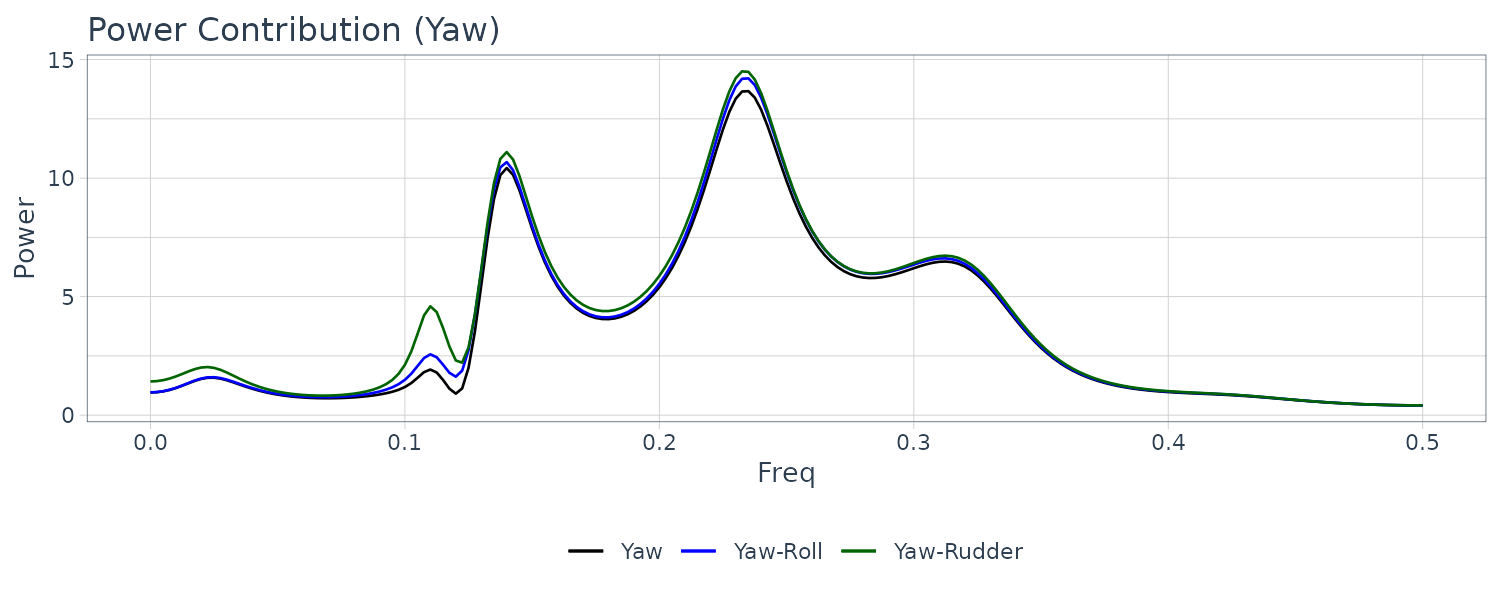
The influence of the rudder angle is clearly visible for \(f < 0.13\). However, the influence of the rudder angle is barely noticeable in the vicinity of \(f = 0.14\) and \(f = 0.23\), where the dominant power of the yaw rate is found. This is probably explained by noting that this data set has been observed under the control of a conventional PID autopilot system that is designed to suppress the power of variation in the frequency area \(f < 0.13\).
The contribution of the rudder angle is almost 50 percent in the vicinity of \(f = 0.1\) where the power spectrum is significant. This is thought to be a side effect of the steering to suppress the variation of the yaw rate. On the other hand, for \(f > 0.14\), a strong influence of the yaw rate is seen, although the actual power is very small.
It can be seen that the influence of the yaw rate is very strong in the vicinity of \(f = 0.12\) where the power spectrum is large. Moreover, it can also be seen that in the range of \(f < 0.08\), the contribution of the yaw rate becomes greater as the frequency decreases.
Fitting an AR Model
Given a time series \(y_{1}, \cdots, y_{N}\), we consider the problem of fitting an autoregressive model (AR model):
\[\begin{aligned} y_{n} &= \sum_{i=1}^{m}a_{i}y_{n-i} + v_{n} \end{aligned}\]To identify an AR model, it is necessary to determine the order m and estimate the autoregressive coefficients \(a_{1}, \cdots, a_{m}\) and the variance \(\sigma^{2}\) from the data.
\[\begin{aligned} \boldsymbol{\theta} &= \begin{bmatrix} a_{1}\\ \vdots\\ a_{m}\\ \sigma^{2} \end{bmatrix} \end{aligned}\]\(\sigma^{2}\) is often called the innovation variance.
Under the assumption that the order m is given, consider the estimation of the parameter \(\boldsymbol{\theta}\) by the maximum likelihood method. The joint distribution of time series:
\[\begin{aligned} \textbf{y} &= \begin{bmatrix} y_{1}\\ \vdots\\ y_{N} \end{bmatrix} \end{aligned}\]Becomes a multivariate normal distribution.
The mean vector of the autoregressive process:
\[\begin{aligned} E[\textbf{y}] &= \textbf{0} \end{aligned}\]And the variance-covariance matrix is given by:
\[\begin{aligned} \boldsymbol{\Sigma} &= \begin{bmatrix} C_{0} & C_{1} & \cdots & C_{N-1}\\ C_{1} & C_{0} & \cdots & C_{N-2}\\ \vdots & \vdots & \ddots & \vdots\\ C_{N-1} & C_{N-2} & \cdots & C_{0} \end{bmatrix} \end{aligned}\]The likelihood of the AR model is obtained by:
\[\begin{aligned} L(\boldsymbol{\theta}) &= p(y_{1}, \cdots, y_{N}|\boldsymbol{\theta})\\ &= \frac{1}{\sqrt{(2\pi)^{2}|\boldsymbol{\Sigma}|}}e^{-\frac{1}{2}\textbf{y}^{T}\boldsymbol{\Sigma}^{-1}\textbf{y}} \end{aligned}\]However, when the number of data, N, is large, the computation of the likelihood by this method becomes difficult because it involves the inversion and computation of the determinant of the \(N \times N\) matrix \(\boldsymbol{\Sigma}\). Further, to obtain the maximum likelihood estimate of \(\boldsymbol{\theta}\), it is necessary to apply a numerical optimization method, since the likelihood is a complicated function of the parameter.
In general, however, the likelihood of a time series model can be efficiently calculated by expressing it as a product of conditional distributions:
\[\begin{aligned} L(\boldsymbol{\theta}) &= p(y_{1}, \cdots, y_{N}|\boldsymbol{\theta})\\ &= p(y_{N}|y_{1}, \cdots, y_{N-1}, \boldsymbol{\theta})p(y_{1}, \cdots, y_{N-1}|\boldsymbol{\theta})\\ &= p(y_{N}|y_{1}, \cdots, y_{N-1}, \boldsymbol{\theta})p(y_{N-1}|y_{1}, \cdots, y_{N-2}, \boldsymbol{\theta})p(y_{1}, \cdots, y_{N-2}|\boldsymbol{\theta})\\ &\ \ \vdots\\ &= p(y_{1}, \boldsymbol{\theta})\prod_{n=2}^{N}p(y_{n}|y_{1}, \cdots, y_{n-1}, \boldsymbol{\theta}) \end{aligned}\]Using a Kalman filter, each term in the right-hand side can be efficiently and exactly evaluated, which makes it possible to compute the exact likelihood of the ARMA model and other time series models.
The AIC for the model is defined by:
\[\begin{aligned} \text{AIC} &= -2 \log L(\hat{\boldsymbol{\theta}}) + 2(m+1) \end{aligned}\]Yule-Walker Method
As shown previously, the autocovariance function of the AR of order m satisfies the Yule-Walker equation:
\[\begin{aligned} C_{0} &= \sum_{i=1}^{m}a_{i}C_{i} + \sigma^{2}\\ C_{j} &= \sum_{i=1}^{m}a_{i}C_{j-1} \end{aligned}\]By computing the sample autocovariance functions \(\hat{C}_{k}\) and substituting them into above equations, we obtain a system of linear equations for the unknown autoregressive coefficients \(a_{1}, \cdots, a_{m}\):
\[\begin{aligned} \begin{bmatrix} \hat{C}_{0} & \hat{C}_{1} & \cdots \hat{C}_{m-1}\\ \hat{C}_{1} & \hat{C}_{0} & \cdots \hat{C}_{m-2}\\ \vdots & \vdots & \ddots & \vdots\\ \hat{C}_{m-1} & \hat{C}_{m-2} & \cdots \hat{C}_{0} \end{bmatrix} \begin{bmatrix} a_{1}\\ a_{2}\\ \vdots\\ a_{m} \end{bmatrix} &= \begin{bmatrix} \hat{C}_{1}\\ \hat{C}_{2}\\ \vdots\\ \hat{C}_{m} \end{bmatrix} \end{aligned}\]The estimates \(\hat{a}_{i}\) of the AR coefficients are obtained by solving this equation. Then from the Yule-Walker equations, an estimate of the variance is obtained by:
\[\begin{aligned} \hat{\sigma}^{2} &= \hat{C}_{0} - \sum_{i=1}^{m}\hat{a}_{i}\hat{C}_{i} \end{aligned}\]We can also obtain the following Yule-Walker equation from minimizing the prediction errors:
\[\begin{aligned} C_{j} &= \sum_{i=1}^{m}a_{i}C_{j-i} \end{aligned}\] \[\begin{aligned} E[v_{n}^{2}] &= E[(y_{n}- \sum_{i=1}^{m}a_{i}y_{n-i})^{2}]\\ &= C_{0} - 2\sum_{i=1}^{m}a_{i}C_{i} + \sum_{i=1}^{m}\sum_{j=1}^{m}a_{i}a_{j}C_{i-j} \end{aligned}\] \[\begin{aligned} \frac{\partial E[v_{n}^{2}]}{\partial a_{j}} &= -2C_{j} + 2\sum_{i=1}^{m}a_{i}C_{j-i} &= 0 \end{aligned}\]Levinson’s Algorithm
To obtain the Yule-Walker estimates for an AR model of order m, it is necessary to solve a system of linear equations with m unknowns. In addition, to select the order of the AR model by the minimum AIC method, we need to evaluate the AIC values of the models with orders up to the maximum order, M. Namely, we have to estimate the coefficients by solving systems of linear equations with 1 unknown, …, M unknowns.
However, by the Levinson’s algorithm, these solutions can be obtained quite efficiently. Hereafter, the AR coefficients and the innovation variance of the AR model of order m are denoted as \(a_{j}^{m}\) and \(\sigma_{m}^{2}\),respectively.
Then Levinson’s algorithm is defined as follows:
Set:
\[\begin{aligned} \hat{\sigma}_{0}^{2} &= \hat{C}_{0} \end{aligned}\] \[\begin{aligned} \text{AIC}_{0} &= N(\log 2\pi\hat{\sigma}_{0}^{2} + 1) + 2 \end{aligned}\]For \(m = 1, \cdots, M\)
\[\begin{aligned} \hat{a}_{m}^{m} &= \frac{\hat{C}_{m} - \sum_{j=1}^{m-1}\hat{C}_{m-j}}{\hat{\sigma}_{m-1}} \end{aligned}\]Recall \(\hat{a}_{m}^{m}\) is the PARCOR.
Calculate \(a_{i}\) from \(i = 1, \cdots, m-1\):
\[\begin{aligned} \hat{a}_{i}^{m} &= \hat{a}_{i}^{m-1} - \hat{a}_{m}^{m}\hat{a}_{m-i}^{m-1} \end{aligned}\] \[\begin{aligned} \hat{\sigma}_{m}^{2} &= \hat{\sigma}_{m-1}^{2}[1 - (\hat{a}_{m}^{m})^{2}] \end{aligned}\] \[\begin{aligned} \text{AIC}_{m} &= N(\log 2\pi \hat{\sigma}_{m}^{2} + 1) + 2(m+1) \end{aligned}\]Derivation of Levinson’s Algorithm
For multivariate time series, the coefficients of the backward AR model are different from those of the forward AR model, the algorithm needs to treat twice as many number of recursions as the univariate case.
Assume that the autocovariance function \(C_{k}\), \(k = 0, 1, \cdots\) is given and that the Yule-Walker estimates of the AR model of order m − 1 have already been obtained.
In the following, since we consider AR models with different orders, the AR coefficients, the prediction error and the prediction error variance of the AR model of order m − 1 are denoted by \(\hat{a}_{1}^{m-1}, \cdots, \hat{a}_{m-1}^{m-1},v_{n}^{m-1},\hat{\sigma}_{m-1}^{2}\).
Since the coefficients \(\hat{a}_{1}^{m-1}, \cdots, \hat{a}_{m-1}^{m-1}\) satisfy the following Yule-Walker equation of order m-1, we have:
\[\begin{aligned} C_{k} &= \sum_{j=1}^{m-1}\hat{a}_{j}^{m-1}C_{j-k} \end{aligned}\] \[\begin{aligned} k &= 1, \cdots, m-1 \end{aligned}\]This means that \(v_{n}^{m-1}\) satisfies:
\[\begin{aligned} E[v_{n}^{m-1}y_{n-k}] &= E[(y_{n} - \sum_{j=1}^{m-1}\hat{a}_{j}^{m-1}y_{n-j})y_{n-k}] = 0 \end{aligned}\] \[\begin{aligned} k &= 1, \cdots, m-1 \end{aligned}\]Now we consider a backward AR model of order m − 1 that represents the present value of the time series yn with future values \(y_{n+1}, \cdots, y_{n+m−1}\):
\[\begin{aligned} y_{n} &= \sum_{i=1}^{m-1}a_{j}y_{n+i} + w_{n}^{m-1} \end{aligned}\]Then, since \(C_{−k} = C_{k}\) holds for a univariate time series, this backward AR model also satisfies the same Yule-Walker equation. Therefore, the backward prediction error \(w_{n}^{m−1}\) satisfies:
\[\begin{aligned} y_{n-m} &= \sum_{i=1}^{m-1}a_{j}y_{n-m+i} + w_{n-m}^{m-1} \end{aligned}\] \[\begin{aligned} E[w_{n-m}^{m-1}y_{n-k}] &= E[(y_{n-m} - \sum_{j=1}^{m-1}\hat{a}_{j}^{m-1}y_{n-m +j})y_{n-k}] = 0 \end{aligned}\] \[\begin{aligned} k &= 1, \cdots, m-1 \end{aligned}\]Now, we define the weighted sum of the forward prediction error \(v_{n}^{m−1}\) and the backward prediction error \(w_{n-m}^{m−1}\) by:
\[\begin{aligned} z_{n} &= v_{n}^{m-1} - \beta w_{n-m}^{m-1}\\ &= y_{n} - \sum_{j=1}^{m-1}\hat{a}_{j}^{m-1}y_{n-j} - \beta\Big(y_{n-m} - \sum_{j=1}^{m-1}\hat{a}_{j}^{m-1}y_{n-m+j}\Big)\\ &= y_{n} - \sum_{j=1}^{m-1}[\hat{a}_{j}^{m-1} - \beta \hat{a}_{m-j}^{m-1}]y_{n-j} - \beta y_{n-m} \end{aligned}\]\(z_{n}\) is a linear combination of \(y_{n}, y_{n−1}, \cdots, y_{n−m}\) and from:
\[\begin{aligned} E[v_{n}^{m-1}y_{n-k}] &= 0\\ E[w_{n-m}^{m-1}y_{n-k}] &= 0 \end{aligned}\]It follows that:
\[\begin{aligned} E[z_{n}y_{n-k}] &= 0 \end{aligned}\] \[\begin{aligned} k = 1, \cdots, m-1 \end{aligned}\]Therefore, if the value of \(\beta\) is determined so that \(E(z_{n}y_{n−m}) = 0\) holds for k = m, the Yule-Walker equation of order m will be satisfied:
\[\begin{aligned} E[z_{n}y_{n-m}] &= E\Big[y_{n} - \sum_{j=1}^{m-1}\hat{a}_{j}^{m-1}y_{n-j} - \beta\Big(y_{n-m} - \sum_{j=1}^{m-1}y_{n-m+j}\Big)\Big]y_{n-m}\\ &= C_{m} - \sum_{j=1}^{m-1}\hat{a}_{j}^{m-1}C_{m-j} - \beta(C_{0} - \sum_{j=1}^{m-1}\hat{a}_{j}^{m-1}C_{j})\\ &= 0 \end{aligned}\]\(\beta\) is then determined as:
\[\begin{aligned} \beta &= \frac{C_{m} - \sum_{j=1}^{m-1}\hat{a}_{j}^{m-1}C_{m-j}}{C_{0} - \sum_{j=1}^{m-1}\hat{a}_{j}^{m-1}C_{m-j}}\\[5pt] &= \frac{C_{m} - \sum_{j=1}^{m-1}\hat{a}_{j}^{m-1}C_{m-j}}{\sigma_{m-1}^{2}} \end{aligned}\]Recall:
\[\begin{aligned} z_{n} &= y_{n} - \sum_{j=1}^{m-1}[\hat{a}_{j}^{m-1} - \beta \hat{a}_{m-1}^{m-1}]y_{n-j} - \beta y_{n-m} \end{aligned}\]If we define \(\beta\) as \(\hat{a}_{m}^{m}\) and \(\hat{a}_{j}^{m}\) as:
\[\begin{aligned} \beta &\equiv \hat{a}_{m}^{m} \end{aligned}\] \[\begin{aligned} \hat{a}_{j}^{m} &\equiv \hat{a}_{j}^{m-1} - \hat{a}_{m}^{m}\hat{a}_{m-j}^{m-1} \end{aligned}\]Then:
\[\begin{aligned} E[z_{n}y_{n-k}] &= E\Big[(y_{n} - \sum_{j=1}^{m}\hat{a}_{j}^{m}y_{n-j})y_{n-k}\Big]\\ &= E[y_{n}y_{n-k}] - \sum_{j=1}^{m}\hat{a}_{j}^{m}y_{n-j}y_{n-k}\\ &= C_{k} - \sum_{j=1}^{m}\hat{a}_{j}^{m}C_{k-j}\\ &= 0 \end{aligned}\] \[\begin{aligned} z_{n} &= y_{n} - \sum_{j=1}^{m-1}[\hat{a}_{j}^{m-1} - \beta \hat{a}_{m-1}^{m-1}]y_{n-j} - \beta y_{n-m}\\ &= y_{n} - \sum_{j=1}^{m}\hat{a}_{j}^{m}y_{n-j} \end{aligned}\]Hence, we get the Yule-Walker equation of order m:
\[\begin{aligned} C_{k} &= \sum_{j=1}^{m}\hat{a}_{j}^{m}C_{k-j}\\ \end{aligned}\] \[\begin{aligned} k = 1, \cdots, m \end{aligned}\]From the Yule-Walker equation, we can express the innovation variance of the AR model as:
\[\begin{aligned} \hat{\sigma}_{m}^{2} &= C_{0} - \sum_{j=1}^{m}\hat{a}_{j}^{m}C_{j}\\ &= C_{0} - \sum_{j=1}^{m}(\hat{a}_{j}^{m-1} - \hat{a}_{m}^{m}\hat{a}_{m-j}^{m-1})C_{j} - \hat{a}_{m}^{m}C_{m}\\ &= C_{0} - \sum_{j=1}^{m}\hat{a}_{j}^{m-1}C_{j} - \hat{a}_{m}^{m}\Bigg(C_{m} - \sum_{j=1}^{m-1}\hat{a}_{m-j}^{m-1}C_{j}\Bigg)\\ &= \hat{\sigma}_{m-1}^{2} - \hat{a}_{m}^{m}\Bigg(C_{m} - \sum_{j=1}^{m-1}\hat{a}_{m-1}^{m-1}C_{j}\Bigg) \end{aligned}\]Recall that:
\[\begin{aligned} \beta &= \hat{a}_{m}^{m}\\ &= \frac{C_{m} - \sum_{j=1}^{m-1}\hat{a}_{m-1}^{m-1}C_{j}}{\hat{\sigma}_{m-1}^{2}} \end{aligned}\] \[\begin{aligned} C_{m} - \sum_{j=1}^{m-1}\hat{a}_{m-1}^{m-1}C_{j} &= \hat{a}_{m}^{m}\hat{\sigma}_{m-1}^{2} \end{aligned}\]Hence:
\[\begin{aligned} \hat{\sigma}_{m}^{2} &= \hat{\sigma}_{m-1}^{2} - \hat{a}_{m}^{m}\Big(C_{m} - \sum_{j=1}^{m-1}\hat{a}_{m-1}^{m-1}C_{j}\Big)\\ &= \hat{\sigma}_{m-1}^{2} - \hat{a}_{m}^{m}(\hat{a}_{m}^{m}\hat{\sigma}_{m-1}^{2})\\[5pt] &= \hat{\sigma}_{m-1}^{2}[1 - (\hat{a}_{m}^{m})^{2}] \end{aligned}\]To show derivation for the AIC, we first note that:
\[\begin{aligned} p(y_{n}|y_{n-1}, \cdots, y_{n-m}) &= -\frac{1}{2}\log 2\pi \sigma_{m}^{2} - \frac{1}{2\sigma_{m}^{2}}\Bigg(y_{n} - \sum_{i=1}^{m}a_{i}y_{n-i}\Bigg)^{2} \end{aligned}\]Hence:
\[\begin{aligned} L(\boldsymbol{\theta}) &= -p(y_{1}, \boldsymbol{\theta})\prod_{n=2}^{N}p(y_{n}|y_{1}, \cdots, y_{n-1}, \boldsymbol{\theta})\\ l(\boldsymbol{\theta}) &= -p(y_{1}, \boldsymbol{\theta}) + \sum_{n=2}^{N}-p(y_{n}|y_{1}, \cdots, y_{n-1}, \boldsymbol{\theta})\\ &= -\frac{N}{2}\log 2\pi \sigma_{m}^{2} - \frac{N}{2\sigma_{m}^{2}}\frac{\sigma_{m}^{2}}{N}\\ &= -\frac{N}{2}\log 2\pi \sigma_{m}^{2} - \frac{1}{2} \end{aligned}\] \[\begin{aligned} \text{AIC}_{m} &= -2l(\boldsymbol{\theta}) + 2(m+1)\\ &= N(\log 2 \pi \hat{\sigma}_{m}^{2} + 1) + 2(m+1) \end{aligned}\]Estimation of an AR Model by the Least Squares Method
The log-likelihood of the AR model:
\[\begin{aligned} l(\boldsymbol{\theta}) &= \sum_{n=1}^{N}\log -p(y_{n}|y_{1}, \cdots, y_{n-1}) \end{aligned}\] \[\begin{aligned} \boldsymbol{\theta} &= \begin{bmatrix} a_{1}\\ \vdots\\ a_{m}\\ \sigma^{2} \end{bmatrix} \end{aligned}\]Here, for the AR model of order m, since the distribution of \(y_{n}\) is specified by the values of \(y_{n−1}, \cdots, y_{n−m}\) for \(n > m\):
\[\begin{aligned} -p(y_{n}|y_{1}, \cdots, y_{n-1}) &= -p(y_{n}|y_{n-m}, \cdots, y_{n-1})\\ &= -\frac{1}{\sqrt{2\pi\sigma^{2}}}e^{-\frac{1}{2\sigma^{2}}(y_{n} - \sum_{i=1}^{m}a_{i}y_{n-i})^{2}} \end{aligned}\]And taking the log:
\[\begin{aligned} - p(y_{n}|y_{n-m}, \cdots, y_{n-1}) &= -\frac{1}{2}\log 2\pi\sigma^{2} - \frac{1}{2\sigma^{2}}(y_{n}- \sum_{i=1}^{m}a_{i}y_{n-i})^{2} \end{aligned}\]Therefore, by ignoring the initial \(M\) (\(M \geq m\)) terms, an approximate log-likelihood of the AR model is obtained as:
\[\begin{aligned} l(\boldsymbol{\theta}) &= \sum_{n = M + 1}^{N}-\log p(y_{n}|y_{n-m}, \cdots, y_{n-1})\\ &= -\frac{N-M}{2}\log 2\pi\sigma^{2} - \frac{1}{2\sigma^{2}}\sum_{n=M+1}^{N}\Bigg(y_{n} - \sum_{i=1}^{m}a_{i}y_{n-i}\Bigg)^{2} \end{aligned}\]Similar to the case of the regression model, for arbitrarily given autoregressive coefficients \(a_{1}, \cdots, a_{m}\), an approximate maximum likelihood estimate of the variance \(\sigma^{2}\) maximizing satisfies:
\[\begin{aligned} \frac{\partial l(\boldsymbol{\theta})}{\partial \sigma^{2}} &= -\frac{N-M}{2\sigma^{2}} + \frac{1}{2(\sigma^{2})^{2}}\sum_{n=M+1}^{N}\Bigg(y_{n} - \sum_{i=1}^{m}a_{i}y_{n-i}\Bigg)^{2} = 0 \end{aligned}\] \[\begin{aligned} \hat{\sigma}^{2} &= \frac{1}{N-M}\sum_{n=M+1}^{N}\Bigg(y_{n} - \sum_{i=1}^{m}a_{i}y_{n-i}\Bigg)^{2} \end{aligned}\]Subsituting this back into the log-likelihood, the the approximate log-likelihood becomes a function of the autoregressive coefficients \(a_{1}, \cdots, a_{m}\):
\[\begin{aligned} l(a_{1}, \cdots, a_{m}) &= -\frac{N-M}{2}\log 2\pi\hat{\sigma}^{2} - \frac{N-M}{2} \end{aligned}\]Here, since the logarithm is a monotone increasing function, maximization of the approximate log-likelihood can be achieved by minimizing the variance \(\hat{\sigma}^{2}\). This means that the approximate maximum likelihood estimates of the AR model can be obtained by the least squares method.
To obtain the least squares estimates of the AR models with orders up to M by the Householder transformation, define the matrix \(\textbf{Z}\) and the vector \(\textbf{y}\) by:
\[\begin{aligned} \mathbf{Z} &= \begin{bmatrix} y_{M} & y_{M-1} & \cdots & y_{1}\\ y_{M + 1} & y_{M} & \cdots & y_{2}\\ \vdots & \vdots & \ddots & \vdots\\ y_{N-1} & y_{N-2} & \cdots & y_{N-M} \end{bmatrix} \end{aligned}\] \[\begin{aligned} \textbf{y} &= \begin{bmatrix} y_{M+1}\\ y_{M+2}\\ \vdots\\ y_{N} \end{bmatrix} \end{aligned}\]Construct the \((N - M)\times (M+1)\) matrix:
\[\begin{aligned} \textbf{X} &= [\textbf{Z}|\textbf{y}]\\ &= \begin{bmatrix} y_{M} & y_{M-1} & \cdots & y_{1} & y_{M+1}\\ y_{M + 1} & y_{M} & \cdots & y_{2} & y_{M+2}\\ \vdots & \vdots & \ddots & \vdots & \vdots\\ y_{N-1} & y_{N-2} & \cdots & y_{N-M} & y_{N} \end{bmatrix} \end{aligned}\]And transform it to an upper triangular matrix by Householder transformation:
\[\begin{aligned} \textbf{HX} &= \begin{bmatrix} \textbf{S}\\ \textbf{0} \end{bmatrix}\\ &= \begin{bmatrix} s_{11} & \cdots & s_{1M} & s_{1, M+1}\\ & \ddots & \vdots & \vdots\\ & & s_{MM} & s_{M, M+1}\\ & & & s_{M+1, M+1}\\ 0 & 0 & 0 & 0 \end{bmatrix} \end{aligned}\]Then, for \(0 \leq j \leq M\), the innovation variance and the AIC of the AR model of order j are obtained by:
\[\begin{aligned} \hat{\sigma}_{j}^{2} &= \frac{1}{N-M}\sum_{i=j+1}^{M+1}s_{i,M+1}^{2}\\[5pt] \text{AIC}_{j} &= (N - M)(\log 2\pi\hat{\sigma}_{j}^{2} + 1) + 2(j+1) \end{aligned}\]Moreover, the least squares estimates of the autoregressive coefficients, which are the solutions of the linear equation:
\[\begin{aligned} \begin{bmatrix} s_{11} & \cdots & s_{1j}\\ & \ddots & \vdots\\ & & s_{jj} \end{bmatrix} \begin{bmatrix} a_{1}\\ \vdots\\ a_{j} \end{bmatrix} &= \begin{bmatrix} s_{1, M+1}\\ \vdots\\ s_{j, M+1} \end{bmatrix} \end{aligned}\]Can be easily obtained by backward substitution as follows:
\[\begin{aligned} \hat{a}_{j} &= \frac{s_{j, M+1}}{s_{jj}}\\ \hat{a}_{i} &= \frac{s_{i,M+1}- s_{i, i+1}\hat{a}_{i+1} - \cdots - s_{i,j}\hat{a_{j}}}{s_{jj}} \end{aligned}\] \[\begin{aligned} i = j-1, \cdots, 1 \end{aligned}\]Estimation of an AR Model by the PARCOR Method
Assuming that the autocovariance functions \(C_{0},C_{1}, \cdots\) are given, Levinson’s algorithm can be executed by using the following relation between the coefficients of the AR model of order m − 1 and the coefficients of the AR model of order m:
\[\begin{aligned} a_{j}^{m} &= a_{j}^{m-1} - a_{m}^{m}a_{m-j}^{m-1} \end{aligned}\]In the derivation of Levinson’s Algorithm section, we shown that:
\[\begin{aligned} \beta &= \hat{a}_{m}^{m}\\ &= \frac{C_{m} - \sum_{j=1}^{m-1}\hat{a}_{m-1}^{m-1}C_{j}}{\hat{\sigma}_{m-1}^{2}} \end{aligned}\]Therefore, if we can estimate the \(a_{m}^{m}\), the other coefficients can be automatically determined by using the above relation. In Levinson’s algorithm, we estimated \(a_{m}^{m}\) by using the following formula that is obtained by substituting the sample autocovariance functions \(\hat{C}_{0}, \cdots, \hat{C}_{m}\):
\[\begin{aligned} \hat{a}_{m}^{m} &= \frac{\hat{C}_{m} - \sum_{j=1}^{m-1}\hat{a}_{j}^{m-1}\hat{C}_{m-j}}{\hat{C}_{0} - \sum_{j=1}^{m-1}\hat{a}_{j}^{m-1}\hat{C}_{j}}\\ &= \frac{\hat{C}_{m} - \sum_{j=1}^{m-1}\hat{a}_{j}^{m-1}\hat{C}_{m-j}}{\hat{\sigma}_{m-1}^{2}} \end{aligned}\]In this section, we present another method of estimating PARCOR \(a_{m}^{m}\) directly from the time series \(y_{1}, \cdots, y_{N}\) without using the sample autocovariance functions.
First of all, let \(w_{n}^{m-1}\) denote the prediction error of the backward AR model with order m − 1:
\[\begin{aligned} y_{n} &= \sum_{j=1}^{m-1}a_{j}^{m-1}y_{n+j} + w_{n}^{m-1} \end{aligned}\]Then:
\[\begin{aligned} y_{n -m} &= \sum_{j=1}^{m-1}a_{j}^{m-1}y_{n-m+j} + w_{n-m}^{m-1} \end{aligned}\]In the case of a univariate time series, since the autocovariance function is an even function, the AR coefficients of the forward model coincide with those of the backward model.
From the Yule-Walker equation:
\[\begin{aligned} C_{m} - \sum_{j=1}^{m-1}a_{j}^{m-1}C_{m-j} &= E\Big[(y_{n} - \sum_{j=1}^{m-1}a_{j}^{m-1}y_{n-j})y_{n-m}\Big]\\ &= E[v_{n}^{m-1}y_{n-m}]\\ &= E[v_{n}^{m-1}\Bigg(\sum_{j=1}^{m-1}a_{j}^{m-1}y_{n-m+j} + w_{n-m}^{m-1}\Bigg)]\\ &= \sum_{j=1}^{m-1}a_{j}^{m-1}E[v_{n}^{m-1}y_{n-m+j}] + E[v_{n}^{m-1}w_{n-m}^{m-1}]\\ &= 0 + E[v_{n}^{m-1}w_{n-m}^{m-1}]\\ &\approx \frac{1}{N-m}\sum_{n=m+1}^{N}v_{n}^{m-1}w_{n-m}^{m-1} \end{aligned}\]On the other hand we can express:
\[\begin{aligned} C_{0} - \sum_{j=1}^{m-1}a_{j}^{m-1}C_{j} &= E[y_{n-m}y_{n-m} - \sum_{j=1}^{m-1}a_{j}^{m-1}y_{n-m+j}y_{n-m}]\\ &= E[(y_{n-m} - \sum_{j=1}^{m-1}a_{j}^{m-1}y_{n-m+j})y_{n-m}]\\ &= E[w_{n-m}^{m-1}y_{n-m}]\\ &= E\Big[w_{n-m}^{m-1}\sum_{j=1}^{m-1}a_{j}^{m-1}y_{n-m+j} + w_{n-m}^{m-1}\Big]\\ &= \sum_{j=1}^{m-1}a_{j}^{m-1}E[w_{n-m}^{m-1}y_{n-m+j}] + E[w_{n-m}^{m-1}w_{n-m}^{m-1}]\\ &= 0 + E[w_{n-m}^{m-1}]^{2}\\ &= E[w_{n-m}^{m-1}]^{2} \end{aligned}\]Since from Yule-Walker equation:
\[\begin{aligned} C_{0} - \sum_{j=1}^{m-1}a_{j}^{m-1}C_{j} &= E[v_{n}^{m-1}]^{2}\\ &= E[w_{n-m}^{m-1}]^{2}\\ &= \sigma^{2} \end{aligned}\]Various estimates of \(E[v_{n}^{m-1}w_{n-m}^{m-1}]\) can be obtained:
\[\begin{aligned} \frac{1}{N-m}\sum_{n=m+1}^{N}(w_{n-m}^{m-1})^{2} \end{aligned}\] \[\begin{aligned} \frac{1}{N-m}\Big[\sum_{n=m+1}^{N}(w_{n-m}^{m-1})^{2} \sum_{n=m+1}^{N}(v_{n}^{m-1})^{2} \Big]^{\frac{1}{2}} \end{aligned}\] \[\begin{aligned} \frac{1}{2(N-m)}\Big[\sum_{n=m+1}^{N}(w_{n-m}^{m-1})^{2} + \sum_{n=m+1}^{N}(v_{n}^{m-1})^{2}\Big] \end{aligned}\]Recall:
\[\begin{aligned} \hat{a}_{m}^{m} &= \frac{\hat{C}_{m} - \sum_{j=1}^{m-1}\hat{a}_{j}^{m-1}\hat{C}_{m-j}}{\hat{C}_{0} - \sum_{j=1}^{m-1}\hat{a}_{j}^{m-1}\hat{C}_{j}} \end{aligned}\] \[\begin{aligned} C_{m} - \sum_{j=1}^{m-1}a_{j}^{m-1}C_{m-j} &\approx \frac{1}{N-m}\sum_{n=m+1}^{N}v_{n}^{m-1}w_{n-m}^{m-1} \end{aligned}\] \[\begin{aligned} C_{0} - \sum_{j=1}^{m-1}a_{j}^{m-1}C_{j} &\approx \frac{\sum_{n = m+1}^{N}w_{n-m}^{m-1}]^{2}}{N-m} \end{aligned}\]Hence we can approximate the PARCOR in 3 ways.
The following estimate is the regression coefficient when the prediction error \(v_{n}^{m-1}\) of the forward model is regressed on the prediction error \(w_{n-m}^{m-1}\) of the backward model.
\[\begin{aligned} \hat{a}_{m}^{m} &= \frac{\sum_{n=m+1}^{N}v_{n}^{m-1}w_{n-m}^{m-1}}{\sum_{n=m+1}^{N}(w_{n-m}^{m-1})^{2}} \end{aligned}\]The following estimate corresponds to the definition of PARCOR, since it is the correlation coefficient of \(v_{n}^{m-1}\) and \(w_{n-m}^{m-1}\):
\[\begin{aligned} \hat{a}_{m}^{m} &= \frac{\sum_{n=m+1}^{N}v_{n}^{m-1}w_{n-m}^{m-1}}{\sqrt{\sum_{n=m+1}^{N}(w_{n-m}^{m-1})^{2}\sum_{n=m+1}^{N}(v_{n-m}^{m-1})^{2}}} \end{aligned}\]The following estimate minimizes the mean of the variances of the forward prediction errors and the backward prediction errors, and consequently Burg’s algorithm based on the maximum entropy method (MEM):
\[\begin{aligned} \hat{a}_{m}^{m} &= 2\frac{\sum_{n=m+1}^{N}v_{n}^{m-1}w_{n-m}^{m-1}}{\sum_{n=m+1}^{N}(w_{n-m}^{m-1})^{2} + \sum_{n=m+1}^{N}(v_{n-m}^{m-1})^{2}} \end{aligned}\]A generic procedure to estimate the AR model from the time series \(y_{1},\cdots, y_{N}\) using the PARCOR method are described below. Here, for simplicity, the mean value of the time series \(y_{n}\) is assumed to be 0:
1) Set:
\[\begin{aligned} v_{n}^{0} &= w_{n}^{0} = y_{n} \end{aligned}\] \[\begin{aligned} n = 1, \cdots, N \end{aligned}\]And compute:
\[\begin{aligned} \hat{\sigma}_{0}^{2} &= \frac{\sum_{n=1}^{N}y_{n}^{2}}{N} \end{aligned}\] \[\begin{aligned} \text{AIC}_{0} &= N(\log 2 \pi \hat{\sigma}_{0} + 1) + 2 \end{aligned}\]2) For \(m = 1, \cdots, M\), repeat the following steps:
(a) Estimate \(\hat{a}_{m}^{m}\) by any of the above 3 formulas.
See the “Estimation of an AR Model by the PARCOR Method” section for above derivation.
(b) Obtain AR coefficients \(\hat{a}_{1}^{m}, \cdots, \hat{a}_{m-1}^{m}\):
\[\begin{aligned} a_{j}^{m} &= a_{j}^{m-1} - a_{m}^{m}a_{m-j}^{m-1} \end{aligned}\](c) For \(n = m + 1, \cdots, N\), obtain the forward prediction error by:
\[\begin{aligned} v_{n}^{m} &= v_{n}^{m-1} - \hat{a}_{m}^{m}w_{n-m}^{m-1} \end{aligned}\](d) For \(n = m + 1, \cdots, N\), obtain the backward prediction error by:
\[\begin{aligned} w_{n-m}^{m} &= w_{n-m}^{m-1} - \hat{a}_{m}^{m}v_{n}^{m-1} \end{aligned}\](e) Estimate the innovation variance of the AR model of order m by:
\[\begin{aligned} \hat{\sigma}_{m}^{2} &= \hat{\sigma}_{m-1}^{2}[1 - (\hat{a}_{m}^{m})^{2}] \end{aligned}\](f) Obtain AIC by:
\[\begin{aligned} \text{AIC}_{m} &= N(\log 2\pi\hat{\sigma}_{m}^{2} + 1) + 2(m+1) \end{aligned}\]Example (AR modeling for sunspot number data)
The function arfit of the package TSSS fits AR model based on the AIC criterion. The method denotes the type of estimation method:
- Yule-Walker method (Default)
- Least squares (Householder) method
- PARCOR method (partial autoregression)
- PARCOR method (PARCOR)
- PARCOR method (Burg’s algorithm)
And the outputs are:
- sigma2: innovation variances
- maice.order: minimum AIC order
- aic: AIC of the AR models
- arcoef: AR coefficients of AR models
- parcor: PARCORs
- spec: power spectrum (in log scale) of the AIC best AR model
fit <- arfit(
  log10(Sunspot$value),
  lag = 20,
  method = 3
)

> names(fit)
[1] "sigma2"  "maice.order"  "aic"  "arcoef"  "parcor"
[6] "spec"    "tsname"
Estimation of Multivariate AR Model by the Yule-Walker Method
\(k\) denotes the number of variables (or dimensions) of a multivariate time series. The parameters of the multivariate AR model with order m:
\[\begin{aligned} \textbf{y}_{n} &= \sum_{i=1}^{m}\textbf{A}_{i}^{m}\textbf{y}_{n-i} + \textbf{v}_{n} \end{aligned}\] \[\begin{aligned} \textbf{v}_{n} &\sim N(\textbf{0}, \textbf{V}_{m}) \end{aligned}\]\(\textbf{V}_{m}\) is the covariance matrix of the innovation \(\textbf{v}_{n}\) and the AR coefficient matrices \(\textbf{A}_{1}^{m}, \cdots, \textbf{A}_{m}^{m}\).
When a multivariate AR model is given, the cross-covariance function is obtained from:
\[\begin{aligned} \textbf{C}_{0} &= \sum_{j=1}^{M}\textbf{A}_{j}\textbf{C}_{-j} + \textbf{W}\\ \textbf{C}_{k} &= \sum_{j=1}^{M}\textbf{A}_{j}\textbf{C}_{k-j} \end{aligned}\] \[\begin{aligned} \textbf{W} &= E[\textbf{v}_{n}\textbf{v}_{n}^{T}]\\ &= \begin{bmatrix} \sigma_{11} & \cdots & \sigma_{1l}\\ \vdots & \ddots &\vdots\\ \sigma_{l1} & \cdots & \sigma_{ll}\\ \end{bmatrix} \end{aligned}\] \[\begin{aligned} k = 1, 2, \cdots \end{aligned}\]On the other hand, using these equations, the estimates of the parameters of the multivariate AR model can be obtained through the sample cross-covariance function.
For actual computation, similarly to the univariate AR model, there is a computationally efficient algorithm. However, for a multivariate time series, the backward model is different from the forward model. In the case of a univariate time series, the forward AR model coincides with the backward AR model, because the autocovariance function is an even function. But this property is not satisfied by multivariate time series. Therefore, in order to derive an efficient algorithm similar to Levinson’s algorithm, we have to consider the backward multivariate AR model:
\[\begin{aligned} \textbf{y}_{n} &= \sum_{i=1}^{m}\textbf{B}_{i}^{m}y_{n+i} + \textbf{u}_{n}\\ \end{aligned}\]And we need to estimate the variance covariance matrix \(\textbf{U}_{m}\) and the coefficients \(\textbf{B}_{i}^{m}\), as well as \(\textbf{V}_{m}\) and \(\textbf{A}_{i}^{m}\) simultaneously.
\[\begin{aligned} \textbf{y}_{n} &= \sum_{i=1}^{m}\textbf{B}_{i}^{m}\textbf{y}_{n+i} + \textbf{u}_{n}\\ \end{aligned}\] \[\begin{aligned} \textbf{u}_{n} &\sim N(\textbf{0}, \textbf{U}_{m}) \end{aligned}\]1) Set:
\[\begin{aligned} \hat{\textbf{V}}_{0} &= \hat{\textbf{U}}_{0} = \textbf{C}_{0} \end{aligned}\]And compute:
\[\begin{aligned} \text{AIC}_{0} &= N(k\log2\pi + \log |\hat{\textbf{V}}_{0}| + k) + k(k + 1) \end{aligned}\]For \(m = 1, \cdots, M\):
a) Set:
\[\begin{aligned} \textbf{W}_{m} &= \textbf{C}_{m}- \sum_{i=1}^{m-1}\textbf{C}_{m-i} \end{aligned}\]b) Obtain the PARCOR matrices of the forward and backward AR models by:
\[\begin{aligned} \textbf{A}_{m}^{m} &= \textbf{W}_{m}\textbf{U}_{m-1}^{-1}\\ \textbf{B}_{m}^{m} &= \textbf{W}_{m}\textbf{V}_{m-1}^{-1}\\ \end{aligned}\]c) Compute the AR coefficients of the forward and backward AR models by:
\[\begin{aligned} \textbf{A}_{m}^{m} &= \textbf{A}_{i}^{m-1} - \textbf{A}_{m}^{m}\textbf{B}_{m-i}^{m-1}\\ \textbf{B}_{m}^{m} &= \textbf{B}_{i}^{m-1} - \textbf{B}_{m}^{m}\textbf{A}_{m-i}^{m-1} \end{aligned}\] \[\begin{aligned} i &= 1, \cdots, m-1 \end{aligned}\]d) Compute the innovation variance covariance matrices by:
\[\begin{aligned} \textbf{V}_{m} &= \textbf{C}_{0} - \sum_{i=1}^{m}\textbf{A}_{i}^{m}\textbf{C}_{i}^{T}\\ \textbf{U}_{m} &= \textbf{C}_{0} - \sum_{i=1}^{m}\textbf{B}_{i}^{m}\textbf{C}_{i} \end{aligned}\]e) Compute the AIC of the AR model of order m by:
\[\begin{aligned} \text{AIC}_{m} &= N(k \log 2\pi + \log |\hat{\textbf{V}}_{m}| + k) + k(k + 1) + 2k^{2}m \end{aligned}\]Example
yy <- HAKUSAN |>
  spread(key = key, value = value) |>
  as_tibble() |>
  select(YawRate, Rolling, Rudder) |>
  as.matrix()

nc <- dim(yy)[1]
n <- seq(1, nc, by = 2)
y <- yy[n, ]

fit <- marfit(y, lag = 20)

> names(fit)
[1] "maice.order"  "aic"  "v" "arcoef"
Estimation of Multivariate AR Model by the Least Squares Method
This least square method has a significant advantage in that we can select a different order for each variable to enable more flexible modeling than the Yule-Walker method. In addition, it is also possible to specify a time-lag for a variable with respect to other variables or to specify a particular coefficient to be zero.
The function marlsq of package TSSS fits multivariate AR models by the least squares method based on the Householder transformation. The highest order of the AR model can be specified by the argument lag. If it is not given, the default value is \(2\sqrt{N}\).
Multivariate AR model was estimated for four-variate HAKUSAN data consisted of yaw rate, rolling, pitching and rudder angle by putting lag=10. The minimum AIC, 6575.741 was attained at m = 10. Using the estimated AR coefficient matrices arcoef and the innovation variance covariance matrix v, the cross-spectrum, coherency and the power contribution are obtained by the function marspc:
yy <- HAKUSAN |>
  spread(key = key, value = value) |>
  as_tibble() |>
  select(Pitching, YawRate, Rolling, Rudder) |>
  as.matrix()

nc <- dim(yy)[1]
n <- seq(1, nc, by = 2)
y <- yy[n, ]

fit <- marlsq(y, lag = 10)
marspc(fit$arcoef, v = fit$v)
Locally Stationary AR Model
Records of real-world phenomena can mostly be categorized as nonstationary time series. The simplest approach to modeling nonstationary time series is to partition the time interval into several subintervals of appropriate size, on the assumption that the time series are stationary on each subinterval. Then, by fitting an AR model to each subinterval, we can obtain a series of models that approximate nonstationary time series.
It is assumed that the time series \(y_{1}, \cdots, y_{N}\) is nonstationary as a whole, but that we can consider it to be stationary on each subinterval of an appropriately constructed partition \((N_{1} + \cdots + N_{k} = N)\). Such a time series that satisfies piecewise stationarity is called a locally stationary time series.
A locally stationary AR model is a nonstationary time series model which has the property that, on each appropriately constructed subinterval, it is stationary and can be modeled by an AR model on each of these subintervals.
Consider the i-th subinterval, \([n_{i0}, n_{i1}]\):
\[\begin{aligned} n_{i0} &= \sum_{j=1}^{i-1}N_{j} +1\\ n_{i1} &= \sum_{j=1}^{i}N_{j} \end{aligned}\]For a locally stationary AR model, the time series \(y_{n}\) follows an AR model on the j-th subinterval:
\[\begin{aligned} y_{n} &= \sum_{i=1}^{m_{j}}a_{ji}y_{n-i} + v_{nj} \end{aligned}\] \[\begin{aligned} E[v_{nj}] &= 0\\ E[v_{nj}^{2}] &= \sigma_{j}%+^{2} \end{aligned}\] \[\begin{aligned} E[v_{nj}y_{n-m}] &= 0 \end{aligned}\] \[\begin{aligned} m &= 1, 2, \cdots \end{aligned}\]The best locally stationary AR model can, in principle, be obtained by the least squares method and AIC. However, practically speaking, it would require an enormous amount of computation to find the model that minimizes the AIC by fitting locally stationary AR models for all possible combinations of numbers of subintervals, k, and data lengths, \(N_{1}, \cdots, N_{k}\). In terms of practice, the following procedure was developed to determine the dividing points of the locally stationary AR model.
Accordingly, only the points \(n_{i} = iL\) are considered as candidates for dividing points, while the minimum unit L of division has been set beforehand. Then, the dividing points of the locally stationary AR model can automatically be decided by the following procedure:
1) Determine the basic span L and the highest order m of the AR models that are fitted to the subinterval of the length L. Here L is set to an appropriate length so that an AR model of order m can be fitted on an interval of length L.
2) Fit AR models of orders up to m to the time series \(y_{1}, \cdots, y_{L}\), and compute \(\text{AIC}_{0}(0), \cdots, \text{AIC}_{m}(0)\) to find \(\text{AIC}_{0} = \mathrm{min}_{j} \text{AIC}_{0}(j)\). Further, set:
\[\begin{aligned} k &= 1\\ n_{10} &= m + 1\\ n_{11} &= L\\ N_{1} &= L − m \end{aligned}\]3) Fit AR models with orders up to m to the time series \(y_{n_{k1} +1}, \cdots, y_{n_{k1} +L}\) and compute \(\text{AIC}_{1}(0), \cdots, \text{AIC}_{1}(m)\) to set \(\text{AIC}_{1} = \textrm{min}_{j} \text{AIC}_{1}(j)\).
\(\text{AIC}_{1}\) is the AIC of a new model that was obtained under the assumption that the model changed at time \(n_{k1} + 1\). The AIC of the locally stationary AR model that divides the interval \([n_{k0}, n_{k1} + L]\) into two subintervals \([n_{k0}, n_{k1}]\) and \([n_{k1} + 1, n_{k1} + L]\) is given by:
\[\begin{aligned} \text{AIC}_{D} &= \text{AIC}_{0} + \text{AIC}_{1} \end{aligned}\]This model is called a divided model.
4) Considering \(y_{n_{k0}}, \cdots, y_{n_{k1}} + L\) to be a stationary interval, fit AR models of orders up to m to compute \(\text{AIC}_{P}(0), \cdots, \text{AIC}_{P}(m)\), and then put \(\text{AIC}_{P} = \textrm{min}_{j} \text{AIC}_{P}(j)\). On the assumption that the time series on the entire interval \([n_{k0}, n_{k1} + L]\) is stationary, the model is called a pooled model.
5) To judge the homogeneity of the two subintervals, compare the \(\text{AIC}_{D}\) of the model of step 3 and the \(\text{AIC}_{P}\) of the model of step 4.
If \(\text{AIC}_{D} < \text{AIC}_{P}\), it is judged that a divided model is better. In this case, \(n_{k1} + 1\) becomes the initial point of the current subinterval and we put:
\[\begin{aligned} k &= k + 1\\ n_{k0} &= n_{k−1,1} + 1\\ n_{k1} &= n_{k−1,1} + L \end{aligned}\] \[\begin{aligned} N_{k} &= L \end{aligned}\]If \(\text{AIC}_{D} \geq \text{AIC}_{P}\), a pooled model is adopted. In this case, the new subinterval \([n_{k1} + 1, n_{k1} + L]\) is merged with the former subinterval, and \([n_{k0}, n_{k1} + L]\) becomes the new current subinterval. Then we put:
\[\begin{aligned} n_{k1} &= n_{k1} + L\\ N_{k} &= N_{k} + L \end{aligned}\] \[\begin{aligned} \text{AIC}_{0} &= \text{AIC}_{P} \end{aligned}\]6) If we have at least L remaining additional data points, we go back to step (3).
Example: (Locally stationary modeling of seismic data)
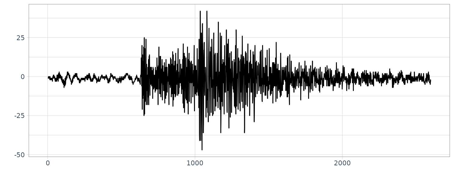
The seismogram record involves microtremors as the noise and two types of seismic wave; the P-wave and the S-wave.
The function lsar of the package TSSS fits locally stationary AR model and automatically divides the time series into several subintervals on which the time series can be considered as stationary.
We fit a locally stationary AR model to the east-west component of a seismogram (N = 2600) with L = 150 and m = 10:
fit <- lsar(
  as.ts(MYE1F),
  max.arorder = 10,
  ns0 = 150
)

> names(fit)
[1]  "model"  "ns"     "span"   "nf"     "ms"
[6]  "sds"    "aics"   "mp"     "sdp"    "aicp"
[11] "spec"   "tsname"
The arguments to be specified are as follows:
- max.arorder: highest order of AR models
- ns0: basic local span.
The outputs from this function are:
- model: = 1: pooled model is accepted, = 2: switched model is accepted.
- ns: number of observations of local spans.
- span: start points and end points of local spans.
- nf: number of frequencies in computing power spectra.
- ms: order of switched model.
- sds: innovation variance of switched model.
- aics: AIC of switched model.
- mp: order of pooled model.
- sdp: innovation variance of pooled model.
- aicp: AIC of pooled model.
- spec: local spectrum.
Plotting the frequency spectrums:
plts <- list()
for (i in seq_along(fit$spec$subspec)) {
  spec <- fit$spec$subspec[[i]]
  n <- length(spec)

  plt <- tibble(
    freq = seq(0, 0.5, length.out = n),
    spec = spec
  ) |>
    ggplot(aes(x = freq, y = spec)) +
    geom_line() +
    ggtitle(
      paste0(
        fit$spec$start[i],
        " - ",
        fit$spec$end[i])
    ) +
    theme_tq()

  plts[[i]] <- plt
}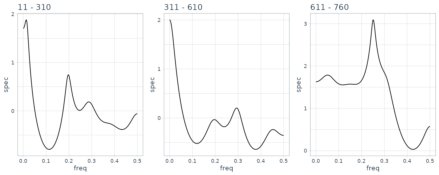
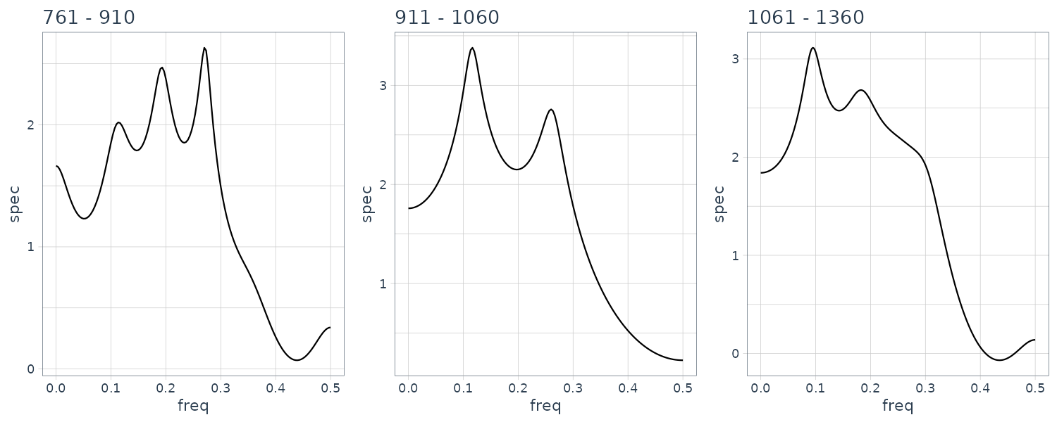
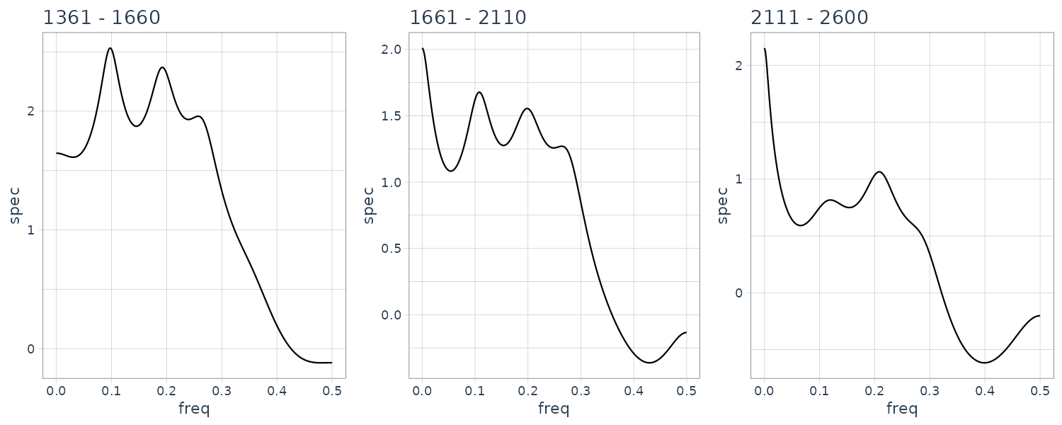
Structural changes have been detected at 8 points, n = 310, 610, 760, 910, 1060, 1360, 1660 and 2010. The change around n = 600 corresponds to a change in the spectrum and the variance caused by the arrival of the P-wave. The section n = 610−910 corresponds to the P-wave. Whereas the spectrum during n = 610 − 760 contains a single strong periodic component, various periodic components with different periods are intermingled during the latter half of the P-wave, n = 760 − 1060. The S-wave appears after n = 1060. We can see not only a decrease in power due to the reduction of the amplitude but also that the main peak shifts from the low frequency range to the high frequency range. After n = 2110, no significant change in the spectrum could be detected.
Precise Estimation of the Change Point
Here, we consider a method of detecting the precise time of a structural change by assuming that a structural change of the time series \(y_{n}\) occurred within the time interval \([n_{0}, n_{1}]\).
Assuming that the structural change occurred at time \(n; n_{0} \leq n \leq n_{1}\), a different AR model is fitted to each subinterval \([1, n − 1]\) and \([n, N]\), respectively. Then the sum of the two AIC’s of the AR models fitted to these time series yields the AIC of a locally stationary AR model with a structural change at time n.
To obtain a precise estimate of the time of structural change based on the locally stationary AR models, we compute the AIC’s for all n such that \(n_{0} \leq n \leq n_{1}\) to find the minimum value. With this method, because we have to estimate AR models for all n, a huge amount of computation is required. However, we can derive a computationally very efficient procedure for obtaining the AIC’s for all the locally stationary AR models by using the method of data augmentation.
Example: Estimation of the arrival times of P-wave and S-wave
The function lsar.chgpt of the package TSSS provides a precise estimate of the time of the structural change of the time series. The required parameters for this function are as follows:
- max.arorder: highest order of AR model.
- subinterval: a vector of the form c(n0,ne), which specifies start and end points of time interval used for modeling.
- candidate: a vector of the form c(n1, n2), which gives the minimum and the maximum for change point. n0+2k < n1 < n2+k < ne, (k is max.arorder)
The outputs from this function are:
- aic: AIC’s of the AR model fitted on [n1,n2].
- aicmin: minimum AIC.
- change.point: estimated change point.
- subint: original sub-interval data.
The first fit exames the change points around \(n = 600\):
fit <- lsar.chgpt(
  as.ts(MYE1F),
  max.arorder = 10,
  subinterval = c(200,1000),
  candidate = c(400,800)
)

> names(fit)
[1] "aic"  "aicmin"  "change.point"  "subint"

> fit$change.point
[1] 630
Plotting the sub-interval from 400 to 800:
MYE1F |>
  slice(fit$subint$st:fit$subint$ed) |>
  autoplot(value) +
  xlab("") +
  ylab("") +
  theme_tq()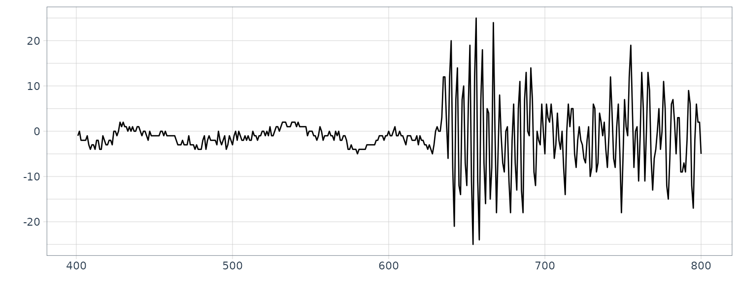
And plotting the change point coinciding with the minimum AIC:
tsibble(
  aic = fit$aic,
  t = fit$subint$st:fit$subint$ed,
  index = t
) |>
  autoplot(aic) +
  geom_text(
    aes(
      y = fit$aicmin,
      x = fit$change.point,
      label = "AIC Min",
      col = "red"
    )
  ) +
  xlab("") +
  ylab("") +
  theme_tq() +
theme(legend.position = "none") 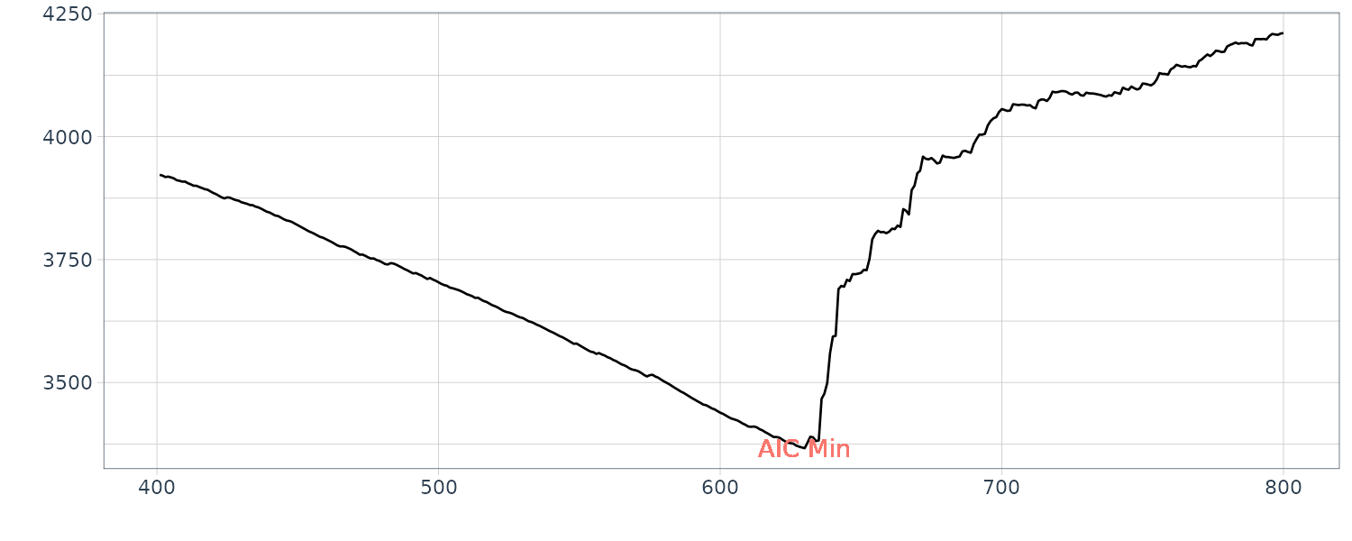
The first half before the change point is considered the micotremors and the latter half is considered the P-wave.
The next change point is around \(n = 1000\):
fit <- lsar.chgpt(
  as.ts(MYE1F),
  max.arorder = 10,
  subinterval = c(600,1400),
  candidate = c(800,1200)
)

> fit$change.point
[1] 1026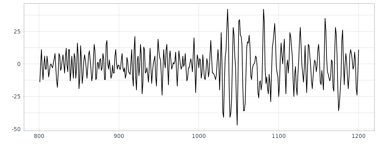
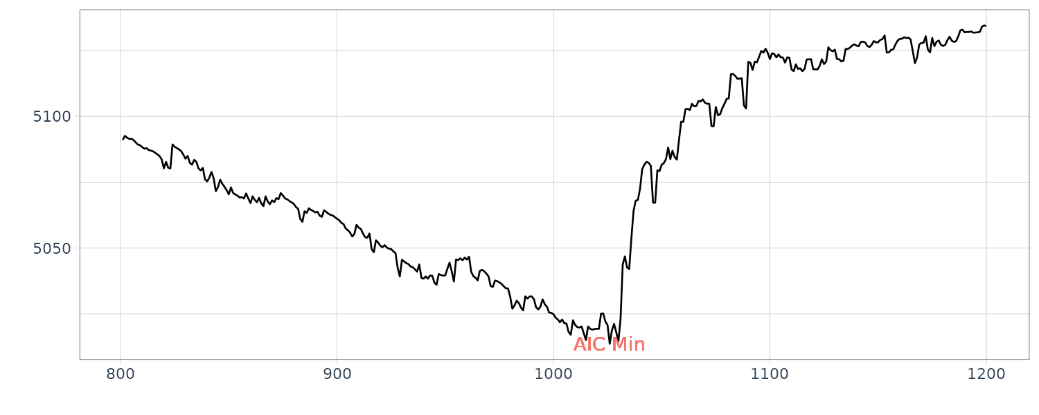
The first half before the second change point is considered the P-wave and latter half the S-wave.
Posterior Probability of the Change Point
It can be shown the likelihood of the model whose parameters are estimated by the maximum likelihood method:
\[\begin{aligned} p(y|j) &= e^{-\frac{1}{2}\text{AIC}_{j}} \end{aligned}\]The above is the likelihood of the LSAR model, which assumes that \(j\) is the arrival time.
Therefore, if the prior distribution of the arrival time is given, then the posterior distribution of the arrival time can be obtained by:
\[\begin{aligned} p(j|y) &= \frac{p(y|j)p(j)}{\sum_{j}p(y|j)p(j)} \end{aligned}\]In the example shown in the next section, the uniform prior over the interval is used. It seems more reasonable to put more weight on the center of the interval. However, since the likelihood, \(p(y\mid j)\), usually takes significant values only at narrow areas, only the local behaviour of the prior is influential to the posterior probability. Therefore as long as very smooth functions are used, the choice of the prior is not so important in the present problem.
fit1 <- lsar.chgpt(
  as.ts(MYE1F),
  max.arorder = 10,
  subinterval = c(400, 800),
  candidate = c(600, 700)
)
AICP <- fit$aic
post <- exp(-(AICP - min(AICP)) / 2)
post <- post / sum(post)

fit2 <- lsar.chgpt(
  as.ts(MYE1F),
  max.arorder = 10,
  subinterval = c(600, 1400),
  candidate = c(800, 1200)
)
AICP2 - fit2$aic
post2 <- exp(-(AICP2 - min(AICP2)) / 2)
post2 <- post / sum(post2)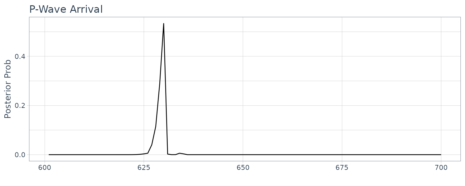
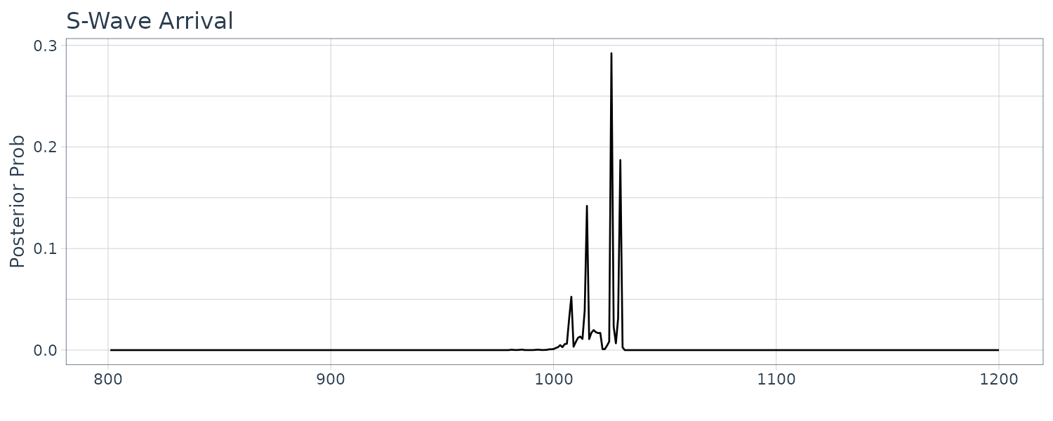
In the case of the arrival of the P-wave, the AIC shown in the middle plot has a clear minimum at about 630. On the other hand, in the case of the arrival of the S-wave, change of the AIC is not so significant and actually has several local minima. Note the difference of the scale of vertical axes in the middle plots. As a result, posterior distribution of the P-wave shown in the left plot has a single peak. On the other hand, that of the S-wave has several peaks.
