Time Series Modeling - State-Space Model
Read PostIn this post, we will continue to cover Kitagawa G. (2021) Introduction to Time Series Modeling focusing on State-Space models.
Contents:
- State-Space Model
- State Estimation via the Kalman Filter
- Smoothing Algorithms
- Long-Term Prediction of the State
- Prediction of Time Series
- Interpolation of Missing Observations
- Trend Model
- Seasonal Adjustment Model
- Time-Varying Variance Model
- Time-Varying Coefficient AR Model
- Non-Gaussian State-Space Model
- See Also
- References
State-Space Model
Various models used in time series analysis can be treated uniformly within the state-space model framework. Many problems of time series analysis can be formulated as the state estimation of a state-space model.
The model for an \(l\)-variate time series \(\textbf{y}_{n}\) consisting of the system model and the observation model as follows is called a state-space model:
\[\begin{aligned} \textbf{x}_{n} &= \textbf{F}_{n}\textbf{x}_{n-1} + \textbf{G}_{n}\textbf{v}_{n} \end{aligned}\] \[\begin{aligned} \textbf{y}_{n} &= \textbf{H}_{n}\textbf{x}_{n} + \textbf{w}_{n} \end{aligned}\] \[\begin{aligned} \textbf{v}_{n} &\sim N(\textbf{0}, \textbf{Q}_{n})\\ \textbf{w}_{n} &\sim N(\textbf{0}, \textbf{R}_{n}) \end{aligned}\]Where \(\textbf{x}_{n}\) is a k-dimensional unobservable vector, referred to as the state. \(\textbf{v}_{n}\) is called a system noise or a state noise and is assumed to be an \(m\)-dimensional white noise with mean vector zero and covariance matrix \(\textbf{Q}_{n}\). On the other hand, \(\textbf{w}_{n}\) is called observation noise and is assumed to be an \(l\)-dimensional Gaussian white noise with mean vector zero and the covariance matrix \(\textbf{R}_{n}\). \(\textbf{F}_{n}, \textbf{G}_{n}, \textbf{H}_{n}\) are \(k \times k\), \(k \times m\), and \(l \times k\) matrices, respectively. Many linear models used in time series analysis are expressible in state-space model.
The state-space model includes the following two typical cases. First, if we consider the observation model as a regression model that expresses a mechanism for obtaining the time series \(\textbf{y}_{n}\), then the state \(\textbf{x}_{n}\) corresponds to the regression coefficients. In this case, the system model expresses the time-change of the regression coefficients.
On the other hand, if the state \(\textbf{x}_{n}\) is an unknown signal, the system model expresses the generation mechanism of the signal, and the observation model represents how the actual observations are obtained, namely they are obtained by transforming the signal and adding observation noise.
Example: State-space representation of an AR model
Consider an AR model for the time series \(y_{n}\):
\[\begin{aligned} y_{n} &= \sum_{i=1}^{m}a_{i}y_{n-i} + v_{n} \end{aligned}\] \[\begin{aligned} v_{n} &\sim (0, \sigma^{2}) \end{aligned}\]Then if \(\textbf{x}_{n}\):
\[\begin{aligned} \textbf{x}_{n} &= \begin{bmatrix} y_{n}\\ y_{n-1}\\ \vdots\\ y_{n-m+1} \end{bmatrix} \end{aligned}\]Then the following state-space model:
\[\begin{aligned} \textbf{x}_{n} &= \textbf{F}\textbf{x}_{n-1} + \textbf{G}_{n}\textbf{v}_{n} \end{aligned}\] \[\begin{aligned} y_{n} &= \textbf{H}_{n}\textbf{x}_{n} + w_{n} \end{aligned}\] \[\begin{aligned} \textbf{F} &= \begin{bmatrix} a_{1} & a_{2} & \cdots & a_{m}\\ 1 & & \cdots & \\ & \ddots & & \\ & & 1 & 0 \end{bmatrix} \end{aligned}\] \[\begin{aligned} \textbf{G} &= \begin{bmatrix} 1\\ 0\\ \vdots\\ 0 \end{bmatrix} \end{aligned}\] \[\begin{aligned} \textbf{H} &= \begin{bmatrix} 1 & 0 & \cdots & 0 \end{bmatrix} \end{aligned}\]Since the first component of the state \(\textbf{x}_{n}\) is the observation \(y_{n}\), by putting \(H = [1, 0, \cdots, 0]\), we obtain the observation model
Therefore, a state-space model representation of the AR model can be obtained by putting \(Q = \sigma^{2}\) and \(R = 0\) to the variances of the system noise and the observation noise, respectively. Thus, the AR model is a special case of the state-space model, in that the state vector \(\textbf{x}_{n}\) is completely determined by the observations until time n, and the observation noise becomes zero.
It should be noted here that the state-space representation of a time series model is not unique, in general. For example, for any regular matrix \(\textbf{T}\):
\[\begin{aligned} \textbf{z}_{n} &= \textbf{T}\textbf{x}_{n}\\ \textbf{F}'_{n} &= \textbf{T}\textbf{F}_{n}\textbf{T}^{-1}\\ \textbf{G}_{n}' &= \textbf{T}\textbf{G}_{n}\\ \textbf{H}_{n}' &= \textbf{H}_{n}\textbf{T}^{-1} \end{aligned}\]We then obtain a state-space model:
\[\begin{aligned} \textbf{z}_{n} &= \textbf{F}'\textbf{z}_{n-1} + \textbf{G}_{n}'\textbf{v}_{n} \end{aligned}\] \[\begin{aligned} \textbf{y}_{n} &= \textbf{H}_{n}'\textbf{z}_{n} +\textbf{w}_{n} \end{aligned}\]In general, many models treated in the book, such as the ARMA model, the trend component model and the seasonal component model, can be expressed in the form:
\[\begin{aligned} \textbf{F} &= \begin{bmatrix} a_{1} & a_{2} & \cdots & a_{m}\\ 1 & & \cdots & \\ & \ddots & & \\ & & 1 & 0 \end{bmatrix} \end{aligned}\] \[\begin{aligned} \textbf{G}_{i} &= \begin{bmatrix} 1\\ b_{1i}\\ \vdots\\ b_{m-1, i} \end{bmatrix} \end{aligned}\] \[\begin{aligned} \textbf{H} &= \begin{bmatrix} c_{1i} & c_{2i} & \cdots & c_{m,i} \end{bmatrix} \end{aligned}\]In actual time series analysis, a composite model that consists of p components is often used. If the dimensions of the p states are \(m_{1}, \cdots, m_{p}\), respectively, with \(m = m_{1} + \cdots + m_{p}\), then by defining an \(m \times m\) matrix, an \(m \times p\) matrix, and an \(m\) vector, a state-space model of the time series is obtained:
\[\begin{aligned} \textbf{F} &= \begin{bmatrix} \textbf{F}_{1} & &\\ & \ddots &\\ & & \textbf{F}_{p} \end{bmatrix} \end{aligned}\] \[\begin{aligned} \textbf{G} &= \begin{bmatrix} \textbf{G}_{1} & &\\ & \ddots &\\ & & \textbf{G}_{p} \end{bmatrix} \end{aligned}\] \[\begin{aligned} \textbf{H} &= \begin{bmatrix} \textbf{H}_{1} & \cdots & \textbf{H}_{p} \end{bmatrix}\\ \end{aligned}\]State Estimation via the Kalman Filter
A particularly important problem in state-space modeling is to estimate the state \(\textbf{x}_{n}\) based on the observations of the time series \(\textbf{y}_{n}\). The reason is that tasks such as prediction, interpolation and likelihood computation for the time series can be systematically performed through the state estimation problem.
In this section, we shall consider the problem of estimating the state \(\textbf{x}_{n}\) based on the set of observations \(\text{Y}_{j} = \{y_{1}, \cdots, y_{j}\}\).
In particular, for \(j < n\), the state estimation problem results in the estimation of the future state based on present and past observations and is called prediction. For \(j = n\), the problem is to estimate the current state and is called a filter. On the other hand, for \(j > n\), the problem is to estimate the past state \(\textbf{x}_{j}\) based on the observations until the present time and is called smoothing.
A general approach to these state estimation problems is to obtain the conditional distribution \(p(\textbf{x}_{n} \mid \textbf{Y}_{j})\) of the state \(\textbf{x}_{n}\) given the observations \(\textbf{Y}_{j}\).
Since the state-space model defined earlier is a linear model and the noises \(\textbf{v}_{n}\) and \(\textbf{w}_{n}\) and the initial state \(\textbf{x}_{0}\) follow normal distributions, all of these conditional distributions become normal distributions. Therefore, to solve the state estimation problem for the state-space model, it is sufficient to obtain the mean vectors and the covariance matrices of the conditional distributions.
In general, in order to obtain the conditional joint distribution of states \(\textbf{x}_{1}, \cdots, \textbf{x}_{n}\) given the observations \(\textbf{y}_{1}, \cdots, \textbf{y}_{n}\), a huge amount of computation is necessary. However, for the state-space model, a very computationally efficient procedure for obtaining the joint conditional distribution of the state has been developed by means of a recursive computational algorithm. This algorithm is known as the Kalman filter.
In the following, the conditional mean and the covariance matrix of the state \(\textbf{x}_{n}\) are denoted by:
\[\begin{aligned} \textbf{x}_{n|j} &= E[\textbf{x}_{n}|\text{Y}_{j}] \end{aligned}\] \[\begin{aligned} \textbf{V}_{n|j} &= E[(\textbf{x}_{n} - \textbf{x}_{n|j})(\textbf{x}_{n} - \textbf{x}_{n|j})^{T}] \end{aligned}\]It is noted that only the conditional distributions with \(j = n − 1\) (one- step-ahead prediction) and \(j = n\) (filter) are treated in the Kalman filter algorithm.
The Kalman filter is realized by repeating the one-step-ahead prediction and the filter with the following algorithms.
One-step-ahead prediction algorithm:
\[\begin{aligned} \textbf{x}_{n|n-1} &= \textbf{F}_{n}\textbf{x}_{n-1|n-1} \end{aligned}\] \[\begin{aligned} \textbf{V}_{n|n-1} &= \textbf{F}_{n}\textbf{V}_{n-1|n-1}\textbf{F}_{n}^{T} + \textbf{G}_{n}\textbf{Q}_{n}\textbf{G}_{n}^{T} \end{aligned}\]Filter algorithm:
\[\begin{aligned} \textbf{K}_{n} &= \textbf{V}_{n|n-1}\textbf{H}_{n}^{T}(\textbf{H}_{n}\textbf{V}_{n|n-1}\textbf{H}_{n}^{T} + \textbf{R}_{n})^{-1} \end{aligned}\] \[\begin{aligned} \textbf{x}_{n|n} &= \textbf{x}_{n|n-1} + \textbf{K}_{n}(\textbf{y}_{n} - \textbf{H}_{n}\textbf{x}_{n|n-1}) \end{aligned}\] \[\begin{aligned} \textbf{V}_{n|n} &= (\textbf{I} - \textbf{K}_{n}\textbf{H}_{n})\textbf{V}_{n|n-1} \end{aligned}\]In the algorithm for one-step-ahead prediction, the predictor (or mean) vector \(\textbf{x}_{n \mid n−1}\) of \(\textbf{x}_{n}\) is obtained by multiplying the transition matrix \(\textbf{F}_{n}\) by the filter of \(\textbf{x}_{n−1}\), \(\textbf{x}_{n−1\mid n−1}\):
\[\begin{aligned} \textbf{x}_{n|n-1} &= \textbf{F}_{n}\textbf{x}_{n-1|n-1} \end{aligned}\]Moreover, the covariance matrix \(\textbf{V}_{n\mid n−1}\) consists of two terms; the first term expresses the influence of the transformation by \(\textbf{F}_{n}\) and the second expresses the influence of the system noise \(\textbf{v}_{n}\):
\[\begin{aligned} \textbf{V}_{n|n-1} &= \textbf{F}_{n}\textbf{V}_{n-1|n-1}\textbf{F}_{n}^{T} + \textbf{G}_{n}\textbf{Q}_{n}\textbf{G}_{n}^{T} \end{aligned}\]In the filter algorithm, the Kalman gain \(\textbf{K}_{n}\) is initially obtained by:
The prediction error of \(\textbf{y}_{n}\):
\[\begin{aligned} \textbf{y}_{n} − \textbf{H}_{n}\textbf{x}_{n | n−1} \end{aligned}\]And the prediction covariance matrices are:
\[\begin{aligned} \textbf{H}_{n}\textbf{V}_{n | n−1}\textbf{H}_{n}^{T} + \textbf{R}_{n} \end{aligned}\]Here, the mean vector of the filter of \(\textbf{x}_{n}\) can be obtained as the sum of the predictor \(\textbf{x}_{n\mid n−1}\) and the prediction error multiplied by the Kalman gain.
Then, since \(\textbf{x}_{n \mid n}\) can be re-expressed as:
\[\begin{aligned} \textbf{x}_{n|n} &= \textbf{K}_{n}\textbf{y}_{n} + (\textbf{I} - \textbf{K}_{n}\textbf{H}_{n})\textbf{x}_{n|n-1} \end{aligned}\]It can be seen that \(\textbf{x}_{n\mid n}\) is a weighted sum of the new observation \(\textbf{y}_{n}\) and the predictor, \(\textbf{x}_{n\mid n−1}\).
The covariance matrix of the filter \(\textbf{V}_{n\mid n}\) can be written as:
\[\begin{aligned} \textbf{V}_{n|n} &= \textbf{V}_{n|n-1} - \textbf{K}_{n}\textbf{H}_{n}\textbf{V}_{n|n-1} \end{aligned}\]Here, the second term of the right-hand side shows the improvement in accuracy of the state estimation of \(\textbf{x}_{n}\) resulting from the information added by the new observation \(\textbf{y}_{n}\).
By using the notation of Hagiwara J. (2021):
Prior distribution:
\[\begin{aligned} \textbf{x}_{0} \sim N(\textbf{m}_{0}, \textbf{C}_{0}) \end{aligned}\]The parameters in the linear Gaussian state space model:
\[\begin{aligned} \boldsymbol{\theta} &= \{\textbf{F}_{n}, \textbf{H}_{n}, \textbf{Q}_{n}, R_{n}, \textbf{m}_{0}, \textbf{C}_{0}\} \end{aligned}\]The filtering distribution, one-step-ahead predictive distribution, and one-step-ahead predictive likelihood are all normal distributions in the Kalman filter. We define them as follows:
Filtering Distribution:
\[\begin{aligned} N(\textbf{x}_{n|n}, \textbf{V}_{n|n}) \end{aligned}\]One-step-ahead Predictive Distribution:
\[\begin{aligned} N(\textbf{x}_{n|n-1}, \textbf{V}_{n|n-1}) \end{aligned}\]One-step-ahead Predictive Likelihood:
\[\begin{aligned} N(p_{n}, P_{n}) \end{aligned}\]Filtering distribution at time point \(t-1\):
\[\begin{aligned} N(\textbf{x}_{n-1|n-1}, \textbf{V}_{n-1|n-1}) \end{aligned}\]Update procedure at time point \(t\)
One-step-ahead predictive distribution:
\[\begin{aligned} \textbf{x}_{n|n-1} &\leftarrow \textbf{F}_{n}\textbf{x}_{n-1|n-1}\\ \end{aligned}\] \[\begin{aligned} \textbf{V}_{n|n-1} &\leftarrow \textbf{F}_{n}\textbf{V}_{n-1|n-1}\textbf{F}_{n}^{T} + \textbf{Q}_{n} \end{aligned}\]One-step-ahead predictive likelihood:
\[\begin{aligned} p_{n} &\leftarrow \textbf{H}_{n}\textbf{x}_{n|n-1} \end{aligned}\] \[\begin{aligned} P_{n} &\leftarrow \textbf{H}_{n}\textbf{V}_{n|n-1}\textbf{H}_{n}^{T} + R_{n} \end{aligned}\]Kalman gain:
\[\begin{aligned} \textbf{K}_{n} &\leftarrow \textbf{V}_{n|n-1}\textbf{H}_{n}^{T}P_{n}^{-1} \end{aligned}\]State update:
\[\begin{aligned} \textbf{x}_{n|n} &\leftarrow \textbf{x}_{n|n-1} + \textbf{K}_{n}(y_{n} - p_{n})\\ \textbf{V}_{n|n} &\leftarrow [\textbf{I} - \textbf{K}_{n}\textbf{H}_{n}]\textbf{V}_{n|n-1} \end{aligned}\]Filtering distribution at time point t:
\[\begin{aligned} N(\textbf{x}_{n|n}, \textbf{V}_{n|n}) \end{aligned}\]Smoothing Algorithms
The problem of smoothing is to estimate the state vector \(\textbf{x}_{n}\) based on the time series \(\textbf{Y}_{m} = \{y_{1}, \cdots, y_{m}\}\) for \(m > n\).
There are three types of smoothing algorithm. If \(m = N\), the smoothing algorithm estimates the state based on the entire set of observations and is called fixed-interval smoothing. If \(n = m − k\), it always estimates the state k steps before, and is called fixed-lag smoothing. If n is set to a fixed time point, e.g. n = 1, it estimates a specific point such as the initial state and is called fixed-point smoothing.
Fixed-interval smoothing
\[\begin{aligned} \textbf{A}_{n} &= \textbf{V}_{n|n}\textbf{F}_{n+1}^{T}\textbf{V}_{n+1}^{-1}\\ \textbf{x}_{n|N} &= \textbf{x}_{n|n} + \textbf{A}_{n}(\textbf{x}_{n+1|N} - \textbf{x}_{n+1|n})\\ \textbf{V}_{n|N} &= \textbf{V}_{n|n} + \textbf{A}_{n}(\textbf{V}_{n+1|N} - \textbf{V}_{n+1|n})\textbf{A}_{n}^{T} \end{aligned}\]The fixed-interval smoothing estimates, \(\textbf{x}_{n\mid N}\) and \(\textbf{V}_{n\mid N}\), can be derived from results obtained by the Kalman filter:
\[\begin{aligned} \textbf{x}_{n|n-1}, \textbf{x}_{n|n}, \textbf{V}_{n|n-1}, \textbf{V}_{n|n} \end{aligned}\]Therefore, to perform fixed-interval smoothing, we initially obtain the above for \(n = 1, \cdots, N\) by the Kalman filter and compute \(\textbf{x}_{N−1\mid N}, \textbf{V}_{N−1\mid N}\) through \(\textbf{x}_{1\mid N}, \textbf{V}_{1\mid N}\) backward in time. It should be noted that the initial values necessary to perform the fixed-interval smoothing algorithm can be obtained by the Kalman filter:
\[\begin{aligned} \textbf{x}_{N|N}, \textbf{V}_{N|N} \end{aligned}\]Again, by using the notation of Hagiwara J. (2021):
\[\begin{aligned} N(\textbf{x}_{n|N}, \textbf{V}_{n|N}) \end{aligned}\]The procedure for obtaining the smoothing distribution at time t from that at time \(t + 1\) is as follows:
Smoothing distribution at time \(t + 1\):
\[\begin{aligned} N(\textbf{s}_{n+1}, \textbf{V}_{n+1|N}) \end{aligned}\]Update procedure at time \(t\):
Smoothing gain:
\[\begin{aligned} \textbf{A}_{n} \leftarrow \textbf{V}_{n|n}\textbf{F}_{n+1}^{T}\textbf{R}_{n+1}^{-1} \end{aligned}\]State update:
\[\begin{aligned} \textbf{x}_{n|N} \leftarrow \textbf{m}_{n} + \textbf{A}_{n}[\textbf{x}_{n+1|N} - \textbf{x}_{n+1|N}]\\ \textbf{V}_{n|N} \leftarrow \textbf{V}_{n|n} + \textbf{A}_{n}[\textbf{V}_{n+1|N} - \textbf{V}_{n+1|n}]\textbf{A}_{n}^{T} \end{aligned}\]Smoothing distribution at time \(t\):
\[\begin{aligned} N(\textbf{x}_{n|N}, \textbf{V}_{n|N}) \end{aligned}\]Long-Term Prediction of the State
It will be shown that by repeating one-step-ahead prediction by the Kalman filter, we can perform long-term prediction, that is, to obtain \(\textbf{x}_{n+k\mid n}\) and \(\textbf{V}_{n+k\mid n}\) for \(k = 1, 2, \cdots\).
Let us consider the problem of estimating the long-term prediction. Firstly, the mean vector \(\textbf{x}_{n+1\mid n}\) and the covariance matrix \(\textbf{V}_{n+1 \mid n}\) of the one-step-ahead predictor of \(\textbf{x}_{n+1}\) are obtained by the Kalman filter.
Here, since the future observation \(\textbf{y}_{n+1}\) is unavailable, it is assumed that \(\textbf{Y}_{n+1} = \textbf{Y}_{n}\). In this case, we have that:
\[\begin{aligned} \textbf{x}_{n+1|n+1} = \textbf{x}_{n+1|n}\\ \textbf{V}_{n+1|n+1} = \textbf{V}_{n+1|n} \end{aligned}\]Therefore, from the one-step-ahead prediction algorithm of the Kalman filter for the period n + 1, we have:
\[\begin{aligned} \textbf{x}_{n+2|n} &= \textbf{F}_{n+2}\textbf{x}_{n+1|n}\\ \textbf{V}_{n+2|n} &= \textbf{F}_{n+2}\textbf{V}_{n+1|n}\textbf{F}_{n+2}^{T} + \textbf{G}_{n+2}\textbf{Q}_{n+2}\textbf{G}_{n+2}^{T} \end{aligned}\]This means that two-step-ahead prediction can be realized by repeating the prediction step of the Kalman filter twice without the filtering step. In general, j-step-ahead prediction based on \(\textbf{Y}_{n}\) can be performed using the relation that \(\textbf{Y}_{n} = \textbf{Y}_{n+1} = \cdots = \textbf{Y}_{n+ j}\) , by repeating the prediction step j times. Summarizing the above, the algorithm for the long-term prediction \(\textbf{x}_{n+1}, \cdots, \textbf{x}_{n+ j}\) based on the observation \(\textbf{Y}_{n}\) can be given as follows:
For \(i = 1, \cdots, j\), repeat:
\[\begin{aligned} \textbf{x}_{n+i|n} &= \textbf{F}_{n+i}\textbf{x}_{n+i-1|n} \end{aligned}\] \[\begin{aligned} \textbf{V}_{n+i|n} &= \textbf{F}_{n+i}\textbf{V}_{n+i-1|n}\textbf{F}_{n+i}^{T} + \textbf{G}_{n+i}\textbf{Q}_{n+i}\textbf{G}_{n+i}^{T} \end{aligned}\]Prediction of Time Series
Future values of time series can be immediately predicted by using the predicted state \(\textbf{x}_{n}\) obtained as shown previously. When \(\textbf{Y}_{n}\) is given, from the relation between the state \(\textbf{x}_{n}\) and the time series \(\textbf{y}_{n}\) which is expressed by the observation model, the mean and the covariance matrix of \(\textbf{y}_{n+ j}\) are denoted by:
\[\begin{aligned} \textbf{y}_{n+j} &= E[\textbf{y}_{n+j}|\textbf{Y}_{n}]\\ \textbf{d}_{n+j} &= \textrm{cov}(\textbf{y}_{n+j}|\textbf{Y}_{n}) \end{aligned}\]Then, we can obtain the mean and the covariance matrix of the j-step-ahead predictor of the time series \(\textbf{y}_{n+j}\) by:
\[\begin{aligned} \textbf{y}_{n+j|n} &= E[\textbf{H}_{n+j}\textbf{x}_{n+j} + \textbf{w}_{n+j}|\textbf{Y}_{n}]\\ &= \textbf{H}_{n+j}\textbf{x}_{n+j|n} \end{aligned}\] \[\begin{aligned} \textbf{d}_{n+j|n} = &\ \textrm{var}(\textbf{H}_{n+j}\textbf{x}_{n+j} + \textbf{w}_{n+j}|\textbf{Y}_{n})\\ = &\ \textbf{H}_{n+j}\textrm{cov}(\textbf{x}_{n+j}|\textbf{Y}_{n})\textbf{H}_{n+j}^{T} + \textbf{H}_{n+j}\textrm{cov}(\textbf{x}_{n+j}, \textbf{w}_{n+j}|\textbf{Y}_{n}) + \\ &\ \textrm{cov}(\textbf{w}_{n+j}, \textbf{x}_{n+j}|\textbf{Y}_{n})\textbf{H}_{n+j}^{T} + \textrm{var}(\textbf{w}_{n+j}|\textbf{Y}_{n})\\ = &\ \textbf{H}_{n+j}\textbf{V}_{n+j|n}\textbf{H}_{n+j}^{T} + \textbf{R}_{n+j} \end{aligned}\]As indicated previously, the predictive distribution of \(\textbf{y}_{n+j}\) based on the observation \(\textbf{Y}_{n}\) of the time series becomes a normal distribution with mean \(\textbf{y}_{n+j\mid n}\) and covariance matrix \(\textbf{d}_{n+j\mid n}\). These are easily obtained above. That is, the mean of the predictor of \(\textbf{y}_{n+j}\) is given by \(\textbf{y}_{n+j\mid n}\), and the standard error is given by \(\textbf{d}_{n+j\mid n}^{\frac{1}{2}}\).
It should be noted that the one-step-ahead predictors \(\textbf{y}_{n\mid n-1}\) and \(\textbf{d}_{n\mid n-1}\) of the time series \(\textbf{y}_{n}\) have already been obtained and were applied in the algorithm for the Kalman filter via the calculation of the Kalman filter and prediction error as shown in the square bracket \([]\) for both the Kalman gain and filtering step below:
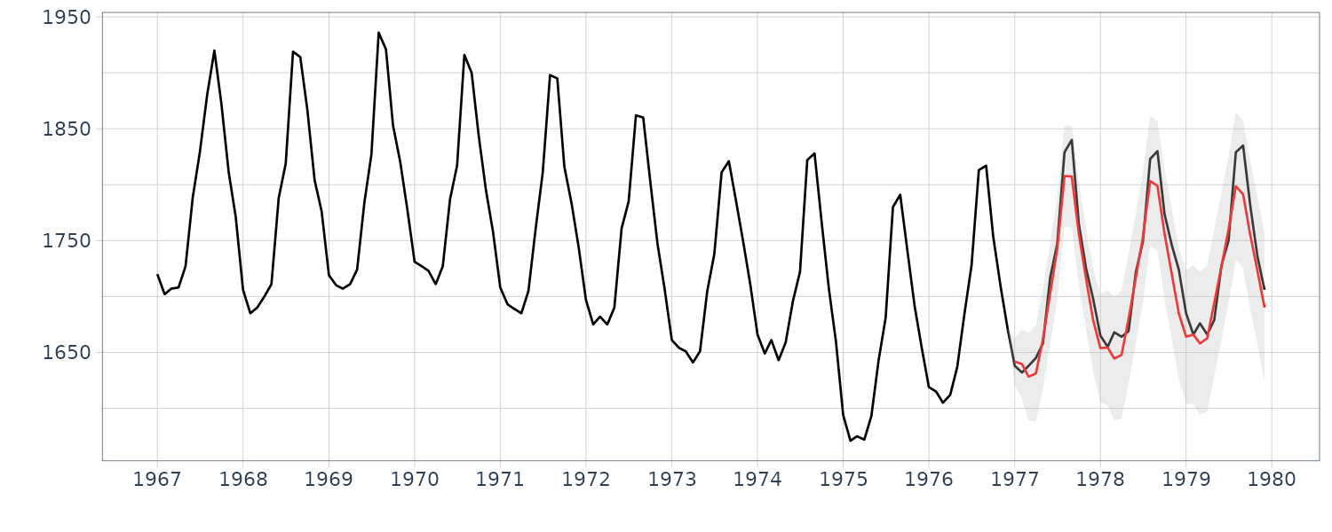
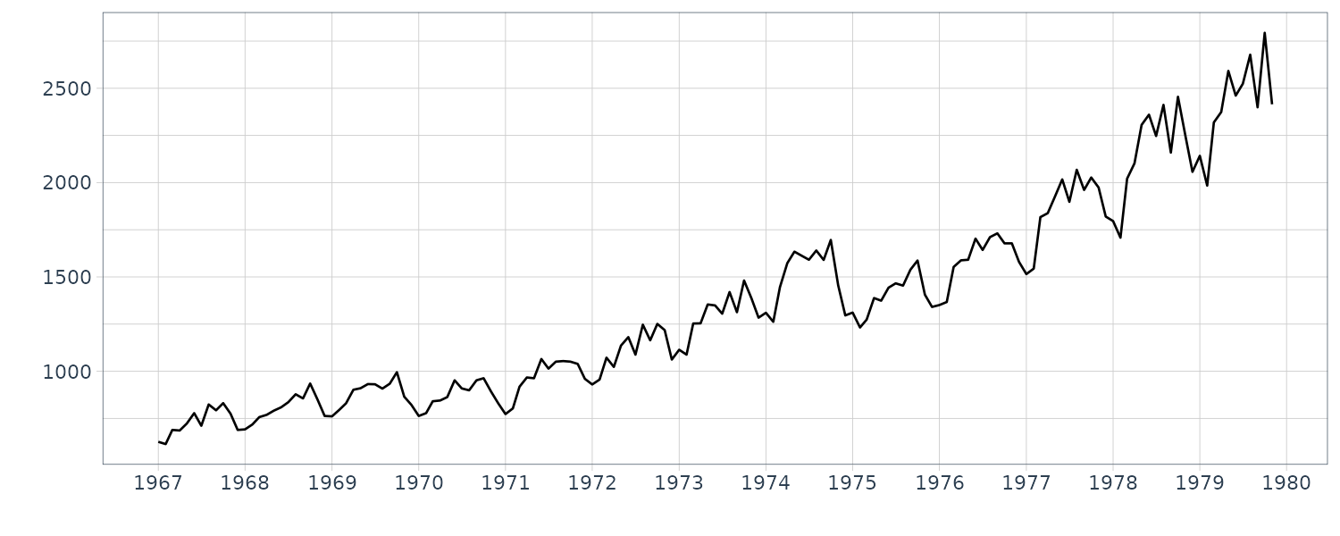
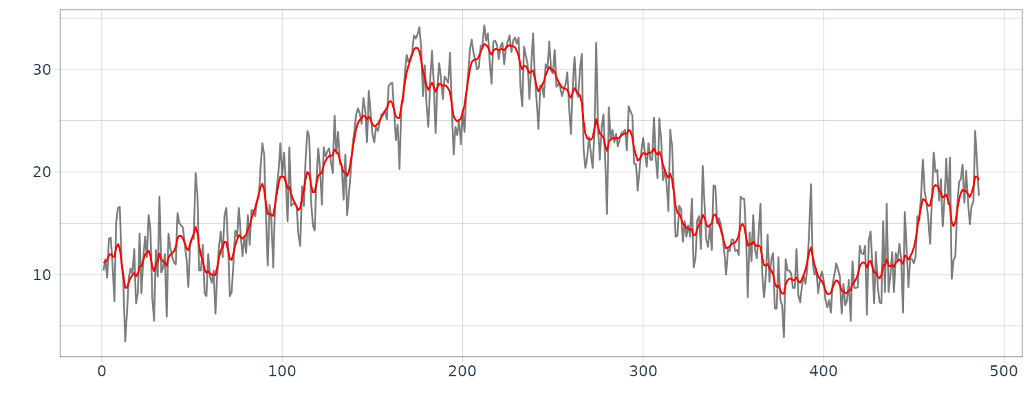
\[\begin{aligned} \textbf{K}_{n} &= \textbf{V}_{n|n-1}\textbf{H}_{n}^{T}([\textbf{H}_{n}\textbf{V}_{n|n-1}\textbf{H}_{n}^{T} + \textbf{R}_{n}])^{-1} \end{aligned}\] \[\begin{aligned} \textbf{x}_{n|n} &= \textbf{x}_{n|n-1} + \textbf{K}_{n}(\textbf{y}_{n} - [\textbf{H}_{n}\textbf{x}_{n|n-1}]) \end{aligned}\]Example: Long-term prediction of BLSALLFOOD data
The function tsmooth of the package TSSS performs long-term prediction by the state-space representation of time series model.
The following arguments are required:
- f: the state transition matrix Fn.
- g: the matrix Gn.
- h: the matrix Hn.
- q: the system noise covariance matrix Qn.
- r: the observation noise variance R.
- x0: initial state vector \(\textbf{x}_{0 \mid 0}\).
- v0: initial state covariance matrix \(\textbf{V}_{0 \mid 0}\).
- filter.end: end point of filtering.
- predict.end: end pont of prediction.
- minmax: lower and upper limit of observations.
And the outputs from this function are:
- mean.smooth: mean vector of smoother.
- cov.smooth: variance of the smoother.
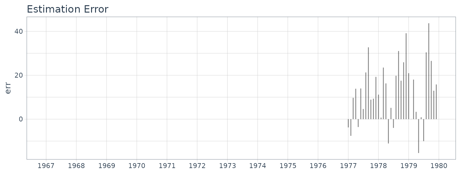
- esterr: estimation error.
- likhood: log-likelihood.
- aic: AIC of the model.
In the following code, an AR model was fitted by the function arfit and the outputs from the function, i.e. the AIC best AR order, the AR coefficients and the innovation variance are used to define the state-space model:
\[\begin{aligned} \textbf{F} &= \begin{bmatrix} a_{1} & a_{2} & \cdots & a_{m}\\ 1 & & \cdots & \\ & \ddots & & \\ & & 1 & 0 \end{bmatrix} \end{aligned}\] \[\begin{aligned} \textbf{G} &= \begin{bmatrix} 1\\ 0\\ \vdots\\ 0 \end{bmatrix} \end{aligned}\] \[\begin{aligned} \textbf{H} &= \begin{bmatrix} 1 & 0 & \cdots & 0 \end{bmatrix} y\end{aligned}\]Note that to perform filtering and long-term prediction by using the AR order different from the AIC best order given in the value z1$maice.order, set m1 to the desired value, such as m1 <- 5.
BLS120 <- BLSALLFOOD$value[1:120] |>
as.ts()
z1 <- arfit(BLS120, plot = FALSE)
> names(z1)
[1] "sigma2" "maice.order" "aic" "arcoef" "parcor"
[6] "spec" "tsname"
tau2 <- z1$sigma2
m1 <- z1$maice.order
arcoef <- z1$arcoef[[m1]]
> arcoef
[1] 1.13164633 -0.13384263 -0.25397419 0.02039985 0.03500777
[6] 0.05990097 -0.17683803 0.08439510 0.10236195 -0.12517702
[11] 0.10852823 0.64089953 -0.74428281 0.04803834 0.15332373
f <- matrix(0.0e0, m1, m1)
f[1, ] <- arcoef
if (m1 != 1) {
for (i in 2:m1) {
f[i, i - 1] <- 1
}
}
g <- c(1, rep(0.0e0, m1-1))
h <- c(1, rep(0.0e0, m1-1))
q <- tau2[m1+1]
r <- 0.0e0
x0 <- rep(0.0e0, m1)
v0 <- NULL
dat <- as.ts(BLSALLFOOD)
# Smoothing by state-space model
s1 <- tsmooth(
dat,
f, g, h, q, r, x0, v0,
filter.end = 120,
predict.end = 156
)
> names(s1)
[1] "mean.smooth" "cov.smooth" "esterr" "llkhood" "aic"
BLSALLFOOD <- BLSALLFOOD |>
mutate(
smooth = s1$mean.smooth[1, ],
sd = sqrt(s1$cov.smooth[1, ]),
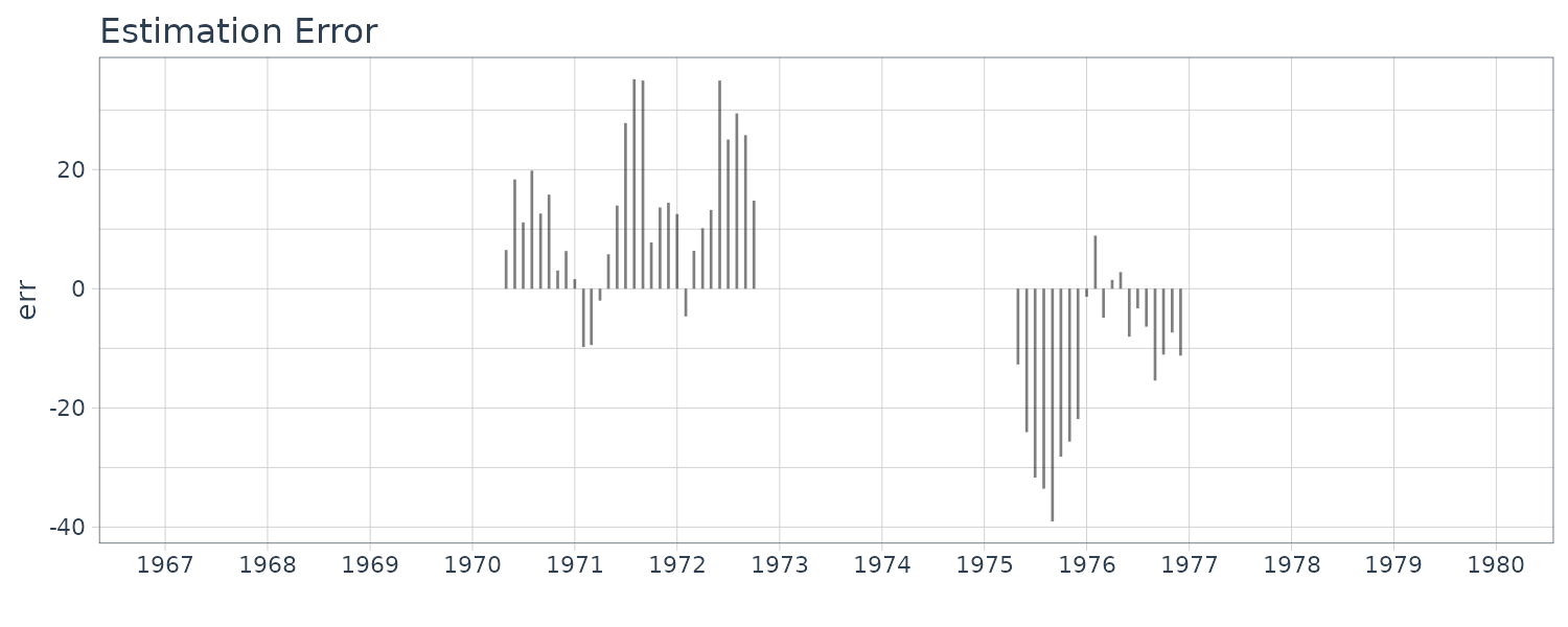
err = s1$esterr
)
Interpolation of Missing Observations
In observing time series, a part of the time series might not be able to be obtained due to unexpected factors such as the breakdown of the observational devices, physical constraints of the observed objects or the observation systems.
In such cases, the actually unobserved data are called missing observations or missing values. Even when only a few percent of the observations are missing, the length of continuously observed data that can be used for the analysis might become very short. In such a situation, we may fill the missing observations with zeros, the mean value of the time series or by linear interpolation. Such an ad hoc interpolation for missing observations may cause a large bias in the analysis, since it is equivalent to arbitrarily assuming a particular model.
If a time series model is given, the model can be used for interpolation of missing observations. Similar to the likelihood computation, firstly we obtain the predictive distributions \(\{\textbf{x}_{n\mid n−1}, \textbf{V}_{n\mid n−1}\}\) and the filter distributions \(\{\textbf{x}_{n\mid n}\), \(\textbf{V}_{n\mid n}\}\) using the Kalman filter and skipping the filtering steps when \(y_{n}\) is missing.
Then we can obtain the smoothed estimates of the missing observations by applying the fixed-interval smoothing algorithm. Consequently, the estimate of the missing observation \(\textbf{y}_{n}\) is obtained by:
\[\begin{aligned} \textbf{y}_{n|N} &= \textbf{H}_{n}\textbf{x}_{n|N} \end{aligned}\]And the covariance matrix of the estimate is obtained by:
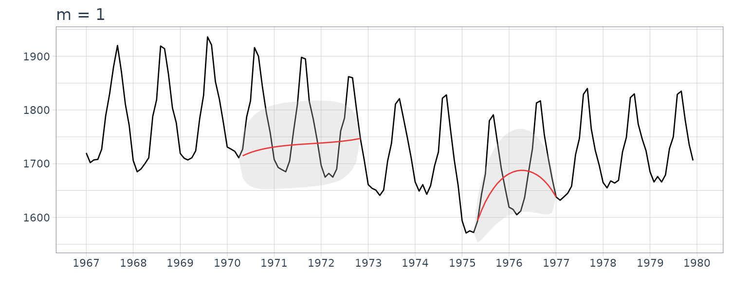
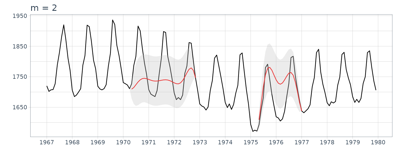
\[\begin{aligned} \textbf{d}_{n|N} = \textbf{H}_{n}\textbf{V}_{n|N} \textbf{H}_{nT} + \textbf{R}_{n} \end{aligned}\]Example: Interpolation of missing observations in BLSALLFOOD data
The function tsmooth of the package TSSS can also compute the log-likelihood of the model for time series with missing observations and interpolate the missing observations based on the state-space representation of the time series model.
Besides the parameters of the state-space model required for long-term prediction, the information about the location of the missing observations is necessary. It can be specified by the arguments missed and np. Here, the vector missed specifies the start position of the missing observations and the vector np specified the number of continuously missing observations.
dat <- as.ts(BLSALLFOOD)

z2 <- arfit(dat, plot = FALSE)
tau2 <- z2$sigma2

# m = maice.order, k=1
m2 <- z2$maice.order
arcoef <- z2$arcoef[[m2]]
f <- matrix(0.0e0, m2, m2)
f[1, ] <- arcoef
if (m2 != 1) {
  for (i in 2:m2) {
    f[i, i - 1] <- 1
  }
}

g <- c(1, rep(0.0e0, m2-1))
h <- c(1, rep(0.0e0, m2-1))
q <- tau2[m2+1]
r <- 0.0e0
x0 <- rep(0.0e0, m2)
v0 <- NULL

s2 <- tsmooth(
  dat,
  f, g, h, q, r, x0, v0,
  missed = c(41,101),
  np = c(30, 20)
)

BLSALLFOOD <- BLSALLFOOD |>
  mutate(
    smooth = s2$mean.smooth[1, ],
    sd = sqrt(s2$cov.smooth[1, ]),
    err = s2$esterr
  )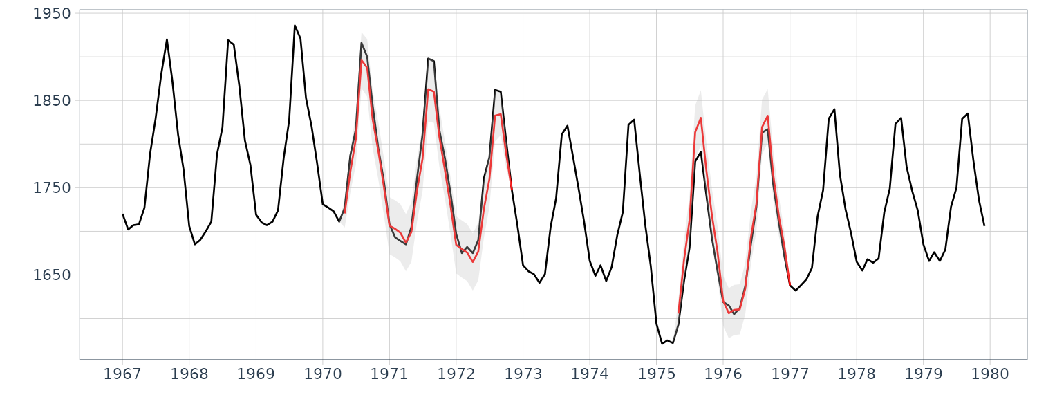
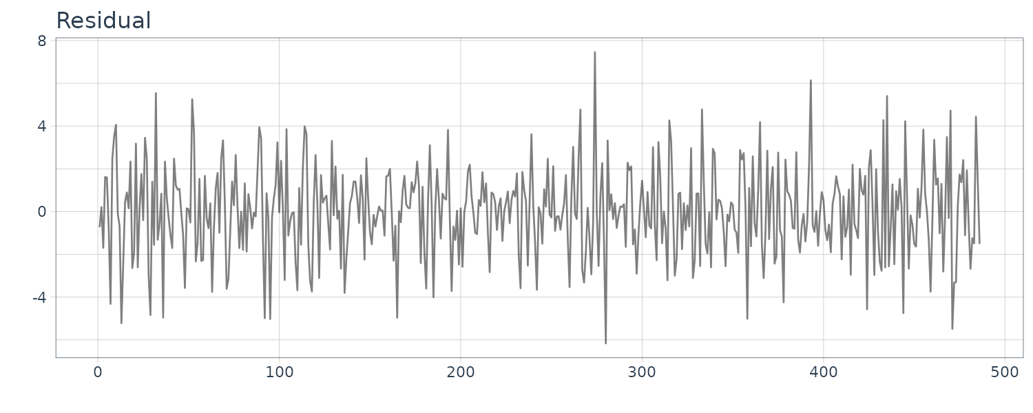
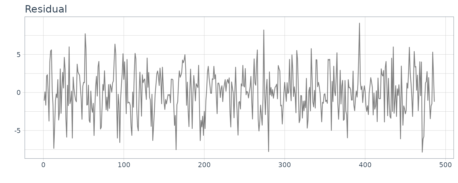
For completion, we also plot for the order \(m = 1\) and \(m = 2\):
Trend Model
Polynomial Trend Model
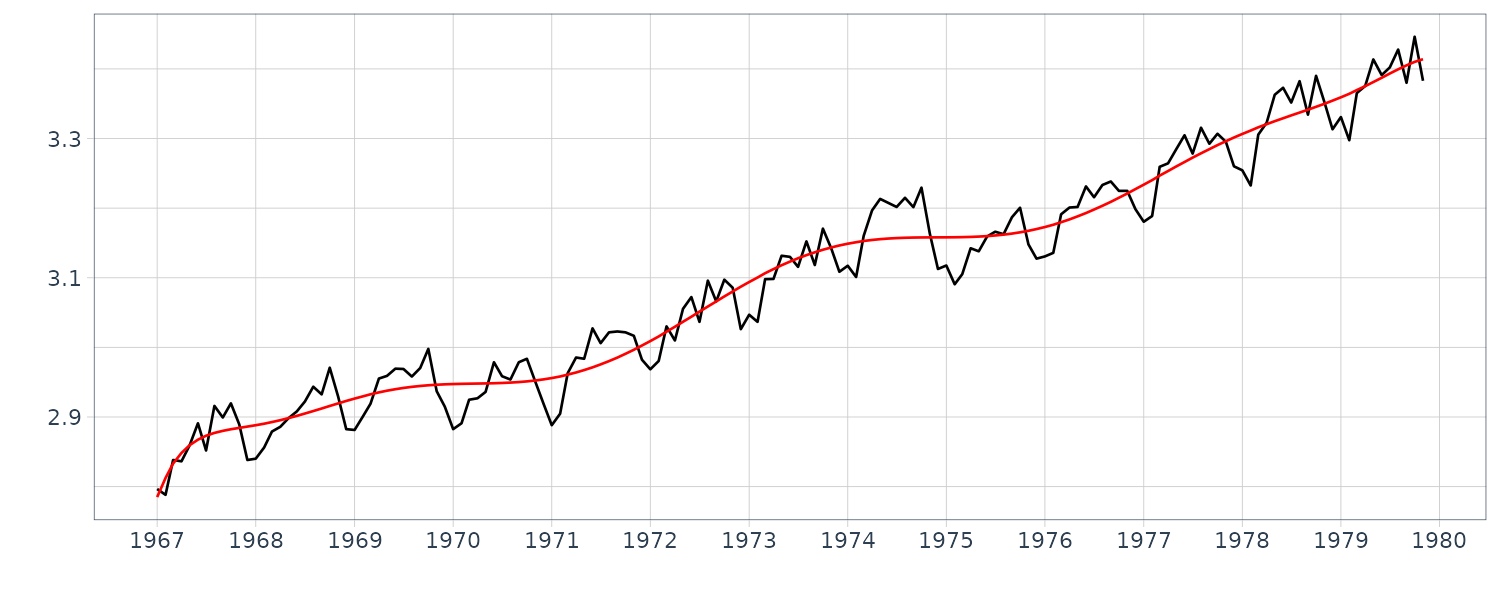
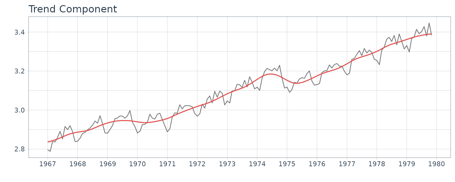
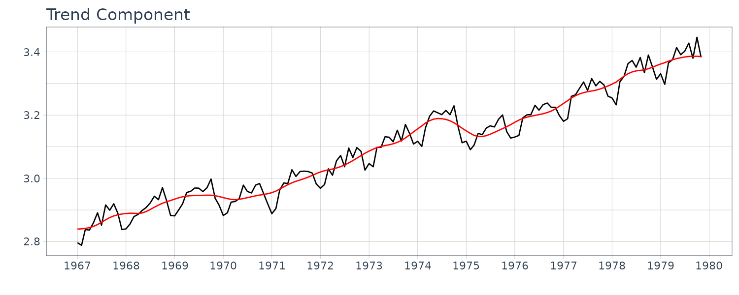
The WHARD data shows a tendency to increase over the entire time domain. Such a long-term tendency often seen in economic time series is called a trend. Needless to say, estimating the trend of such a time series is a very natural way of capturing the tendency of the time series and predicting its future behavior. However, even in the case of analyzing short-term behavior of a time series with a trend, we usually analyze the time series after removing the trend, because it is not appropriate to directly apply a stationary time series model such as the AR model to the original series.
In this section, we shall explain the polynomial regression model as a simple tool to estimate the trend of a time series. For the polynomial regression model, the time series \(y_{n}\) is expressed as the sum of the trend \(t_{n}\) and a residual \(w_{n}\):
\[\begin{aligned} y_{n} &= t_{n} + w_{n} \end{aligned}\]Where \(w_{n}\) follows a Gaussian distribution with mean 0 and variance \(\sigma^{2}\). It is assumed that the trend component can be expressed as a polynomial:
\[\begin{aligned} t_{n}&= a_{0} + a_{1}x_{n} + \cdots + a_{m}x_{n}^{m} \end{aligned}\]To fit a polynomial trend model, we define the j-th explanatory variable as \(x_{nj} = x_{n}^{j−1}\), and construct the matrix \(\textbf{X}\) as:
\[\begin{aligned} \textbf{X} &= \begin{bmatrix} 1 & x_{1} & \cdots x_{1}^{m} & y_{1}\\ \vdots & \vdots & & \vdots & \vdots\\ 1 & x_{N} & \cdots x_{N}^{m} & y_{N} \end{bmatrix} \end{aligned}\]Then, by reducing the matrix \(\textbf{X}\) to an upper triangular form by an appropriate Householder transformation \(\textbf{U}\):
\[\begin{aligned} \textbf{UX} &= \begin{bmatrix} \textbf{S}\\ \textbf{0} \end{bmatrix}\\ &= \begin{bmatrix} s_{11} & \cdots & s_{1,m+2}\\ & \ddots & \vdots\\ & & s_{m+2, m+2}\\ & \textbf{0} & \end{bmatrix} \end{aligned}\]The residual variance of the polynomial regression model of order j is obtained as:
\[\begin{aligned} \hat{\sigma}_{j}^{2} &= \frac{1}{N}\sum_{i=j+2}^{m+2}s_{i,m+2}^{2} \end{aligned}\]Since the j-th order model has j + 2 parameters, i.e., j + 1 regression coefficients and the variance, the AIC is obtained as:
\[\begin{aligned} \text{AIC}_{j} &= N\log 2\pi\hat{\sigma}_{j}^{2} + N + 2(j+2) \end{aligned}\]The AIC best order is then obtained by finding the minimum of the AIC j. Given the AIC best order j, the maximum likelihood estimates of the regression coefficients are obtained by solving the system of linear equations:
\[\begin{aligned} \begin{bmatrix} s_{11} & \cdots & s_{1,m+2}\\ & \ddots & \vdots\\ & & s_{m+2, m+2} \end{bmatrix}\begin{bmatrix} a_{0}\\ \vdots\\ a_{j} \end{bmatrix} &= \begin{bmatrix} s_{1, m+2}\\ \vdots\\ s_{j+1, m+2} \end{bmatrix} \end{aligned}\]R function polreg of the package TSSS fits a polynomial regression model to a time series. The parameter order sp of polynomial regression, and the order of regression is determined by AIC. The function yields the following outputs:ecifies the highest order:
- order.maice: Minimum AIC trend order.
- sigma2: Residual variances of the models with orders \(0 \leq m \leq M\).
- aic: AICs of the models with orders \(0 \leq m \leq M\).
- daic: AIC − min AIC.
- coef: Regression coefficents a(i, m), i = 0, …, m, m = 1, …, M.
- trend: Estimated trend component by the AIC best model.
z <- polreg(dat, order = 9)

> names(z)
[1] "order.maice"  "sigma2"  "aic"  "daic"  "coef" "trend"

y <- WHARD |>
  as.ts() |>
  log10()
z <- polreg(y, order = 15)
names(z)

WHARD <- WHARD |>
  mutate(
    trend = z$trend
  )
The polynomial trend model treated in the previous section can be expressed as:
\[\begin{aligned} y_{n} &\sim N(t_{n}, \sigma^{2}) \end{aligned}\]This type of parametric model can yield a good estimate of the trend, when the actual trend is a polynomial or can be closely approximated by a polynomial. However, in other cases, a parametric model may not reasonably capture the characteristics of the trend, or it may become too sensitive to random noise. Hereafter, we consider a stochastic extension of the polynomial function to mitigate this problem.
Stochastic Extension of Polynomial Function
Consider a polynomial of the first order, i.e. a straight line, given by:
\[\begin{aligned} t_{n} &= an + b \end{aligned}\] \[\begin{aligned} \Delta t_{n} &= a\\ \Delta^{2} t_{n} &= 0 \end{aligned}\]This means that the first order polynomial is the solution of the initial value problem for the second order difference equation:
\[\begin{aligned} \Delta^{2}t_{n} &= 0\\ \Delta t_{0} &= a\\ t_{0} &= b \end{aligned}\]In general, a polynomial of order k − 1 can be considered as a solution of the difference equation of order k:
\[\begin{aligned} \Delta^{k}t_{n} &= 0 \end{aligned}\]In order to make the polynomial more flexible, we assume that \(\Delta^{k} t_{n} \approx 0\) instead of using the exact difference equation. This can be achieved by introducing a stochastic difference equation of order k:
\[\begin{aligned} \Delta^{k}t_{n} &= v_{n} \end{aligned}\] \[\begin{aligned} v_{n} &\sim N(0, \tau^{2}) \end{aligned}\]In the following, we call the model a trend component model. Because the solution of the difference equation \(\Delta^{k} t_{n} = 0\) is a polynomial of order k − 1, the trend component model of order k can be considered as an extension of a polynomial of order k − 1. When the variance \(\tau^{2}\) of the noise is small, the realization of a trend component model becomes locally a smooth function that resembles the polynomial. However, a remarkable difference from the polynomial is that the trend component model can express a very flexible function globally.
Example: Random Walk Model
For k = 1, this model becomes a random walk model, which can be defined by:
\[\begin{aligned} t_{n} &= t_{n-1} + v_{n} \end{aligned}\] \[\begin{aligned} v_{n} &\sim N(0, \tau^{2}) \end{aligned}\]This model expresses that the trend is locally constant and can be expressed as \(t_{n} \approx t_{n−1}\).
For k = 2, the trend component model becomes:
\[\begin{aligned} t_{n} &= 2t_{n-1} - t_{n-2} + v_{n} \end{aligned}\]For which it is assumed that the trend is locally a linear function and satisfies \(t_{n} − 2t_{n−1} + t_{n−2} \approx 0\).
To show this:
\[\begin{aligned} \Delta^{2}t_{n} &= (t_{n} - t_{n-1}) - (t_{n-1} - t_{n-2})\\ &= (2t_{n-1} - t_{n-2} - t_{n-1}) - (t_{n-1} - t_{n-2})\\ &= (t_{n-1} - t_{n-2}) - (t_{n-1} - t_{n-2})\\ &= 0 \end{aligned}\]In general, the k-th order difference operator of the trend component model is given by:
\[\begin{aligned} \Delta^{k} &= (1 - B)^{k}\\ &= \sum_{i=0}^{k}{k\choose i}(-B)^{i} \end{aligned}\]Therefore, using the binomial coefficient:
\[\begin{aligned} c_{i} &= (-1)^{i+1}{k \choose i} \end{aligned}\]The trend component model of order k can be expressed as:
\[\begin{aligned} t_{n} &= \sum_{i=1}^{k}c_{i}t_{n-i} + v_{n} \end{aligned}\]Although these models are not stationary, they can formally be considered as AR models of order k. Note that \(c_{1} = 1\) for \(k = 1\) and \(c_{1} = 2\) and \(c_{2} = −1\) for \(k = 2\). Therefore:
\[\begin{aligned} \textbf{x}_{n} &= \begin{bmatrix} t_{n}\\ t_{n-1}\\ \vdots\\ t_{n-k+1} \end{bmatrix} \end{aligned}\] \[\begin{aligned} \textbf{F} &= \begin{bmatrix} c_{1} & c_{2} & \cdots & c_{k}\\ 1 & & &\\ & \cdots & & \\ & & 1& \end{bmatrix} \end{aligned}\] \[\begin{aligned} \textbf{G} &= \begin{bmatrix} 1\\ 0\\ \vdots\\ 0 \end{bmatrix} \end{aligned}\] \[\begin{aligned} \textbf{H} &= \begin{bmatrix} 1 & 0 & \cdots 0 \end{bmatrix} \end{aligned}\] \[\begin{aligned} \textbf{x}_{n} &= \textbf{F}\textbf{x}_{n-1} + \textbf{G}\textbf{v}_{n} \end{aligned}\] \[\begin{aligned} \textbf{t}_{n} &= \textbf{H}\textbf{x}_{n} \end{aligned}\]Example: State-space representation of trend models
For \(k = 1\):
\[\begin{aligned} x_{n} &= t_{n} \end{aligned}\] \[\begin{aligned} F &= G = H = 1 \end{aligned}\]For \(k = 2\):
\[\begin{aligned} \textbf{x}_{n} &= \begin{bmatrix} t_{n}\\ t_{n-1} \end{bmatrix} \end{aligned}\] \[\begin{aligned} \textbf{F} &= \begin{bmatrix} 2 & -1\\ 1 & 0 \end{bmatrix} \end{aligned}\] \[\begin{aligned} \textbf{G} &= \begin{bmatrix} 1\\ 0 \end{bmatrix} \end{aligned}\] \[\begin{aligned} \textbf{H} &= \begin{bmatrix} 1 & 0 \end{bmatrix} \end{aligned}\]Or:
\[\begin{aligned} \textbf{x}_{n} &= \begin{bmatrix} t_{n}\\ -t_{n-1} \end{bmatrix} \end{aligned}\] \[\begin{aligned} \textbf{F} &= \begin{bmatrix} 2 & 1\\ -1 & 0 \end{bmatrix} \end{aligned}\] \[\begin{aligned} \textbf{G} &= \begin{bmatrix} 1\\ 0 \end{bmatrix} \end{aligned}\] \[\begin{aligned} \textbf{H} &= \begin{bmatrix} 1 & 0 \end{bmatrix} \end{aligned}\]Trend Model
Here, we consider the simplest case where the time series is expressed as:
\[\begin{aligned} \Delta^{k}t_{n} &= v_{n} \end{aligned}\] \[\begin{aligned} y_{n} &= t_{n} + w_{n} \end{aligned}\] \[\begin{aligned} v_{n} &\sim N(0, \tau^{2})\\ w_{n} &\sim N(0, \sigma^{2}) \end{aligned}\]The observation model in equation \(y_{n} = t_{n} + w_{n}\), expresses the situation that the time series \(y_{n}\) is obtained by adding an independent noise to the trend. On the other hand, the trend component model \(\Delta^{k}t_{n} = v_{n}\) expresses the change in the trend. Actual time series are usually not as simple as this and often require more sophisticated modeling as will be treated in the next section.
Based on the state-space representation of the above trend component model, the state-space model of the trend is given as follows:
\[\begin{aligned} \textbf{x}_{n} &= \textbf{F}\textbf{x}_{n-1} + \textbf{Gv}_{n}\\ y_{n} &= \textbf{Hx}_{n} + w_{n} \end{aligned}\]This model differs from the simpler trend component model only in that it contains an additional observation noise.
Once the order k of the trend model and the variances \(\tau^{2}, \sigma^{2}\) have been specified, the smoothed estimates \(\textbf{x}_{1\mid N}, \cdots, \textbf{x}_{N\mid N}\) are obtained by the Kalman filter and the fixed-interval smoothing algorithm.
Since the first component of the state vector is \(t_{n}\), the first component of \(\textbf{x}_{n\mid N}\), namely \(\textbf{Hx}_{n\mid N}\), is the smoothed estimate of the trend \(t_{n\mid N}\).
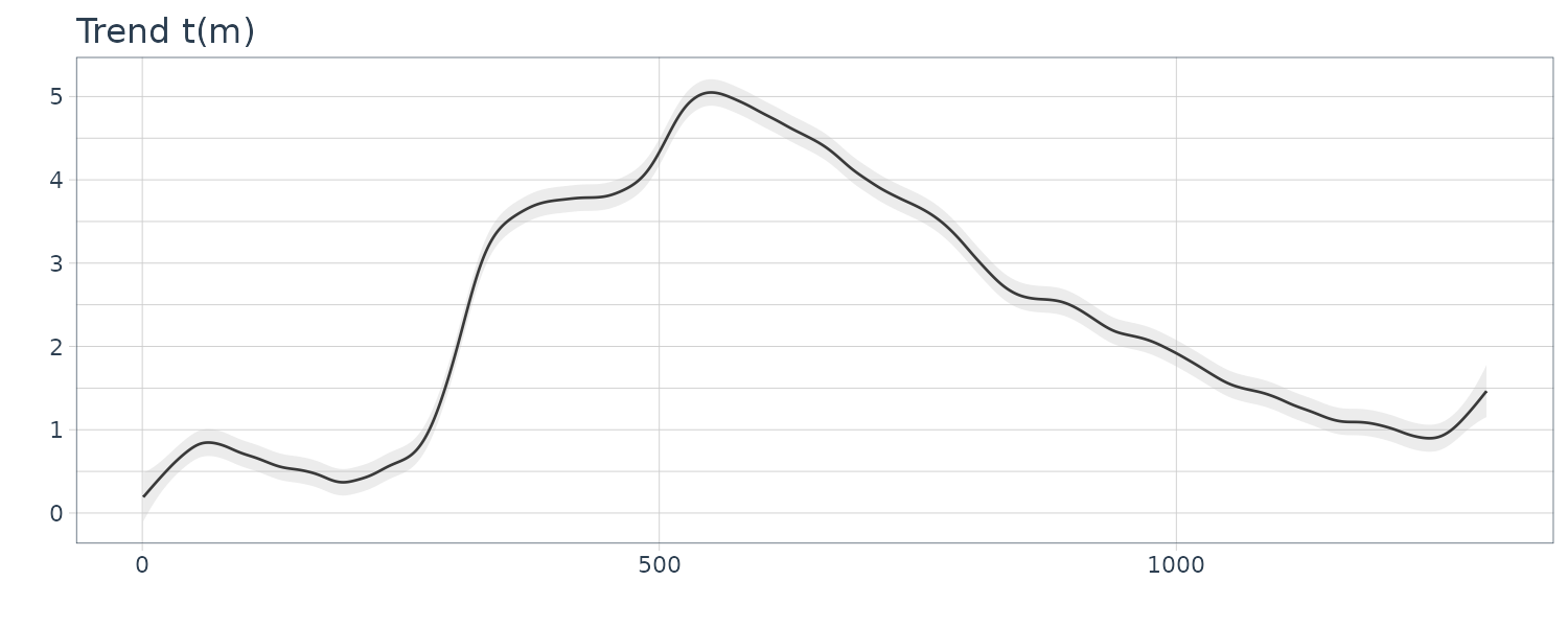
Example: Trend of maximum temperature data
The function trend of the package TSSS fits the trend model and estimates the trend of a time series. The function requires:
- trend.order: the order of the trend component.
- tau2.ini: the initial estimate of the variance of the system noise, \(\tau^{2}\).
- delta: the search width for the \(\tau^{2}\). If tau2=NULL, namely, if an initial estimate of \(\tau^{2}\) is not given, the function yields a rough estimate of \(\tau^{2}\) by searching the smallest AIC within the candidates \(\tau^{2} = 2−k\), \(k = 1, 2, \cdots\).
The function provides the:
- trend: estimated trend.
- residual: residuals.
- tau2: the variance of the system noise \(\tau^{2}\).
- sigma2: the variance of the observation noise \(\sigma^{2}\).
- aic: the log-likelihood of the model (llkhood) and the AIC.
dat <- as.ts(Temperature)
fit <- trend(
  dat,
  trend.order = 1,
  tau2.ini = 0.223,
  delta = 0.001
)

> fit
 tau2 		 2.23000e-01
 sigma2 	 5.54743e+00
 log-likelihood	   -1220.841
 aic		    2447.682

Temperature <- Temperature |>
  mutate(
    trend = fit$trend,
    residual = fit$residual
  )
fit <- trend(
  dat,
  trend.order = 2
)

> fit
 tau2 		 2.44141e-04
 sigma2 	 8.17920e+00
 log-likelihood	   -1248.696
 aic		    2505.392

Temperature <- Temperature |>
  mutate(
    trend = fit$trend,
    residual = fit$residual
  )
We can see that the second order trend model yields a considerably smoother trend. As shown in the above examples, the trend model contains the order k and the variances \(\tau^{2}, \sigma^{2}\) as parameters, which yield a variety of trend estimates.
To obtain a good estimate of the trend, it is necessary to select appropriate parameters. The estimates of the variances \(\tau^{2}, \sigma^{2}\) are obtained by the maximum likelihood method. Comparison of the AIC values for k = 1 and k = 2 reveals that the AIC for k = 1 is significantly smaller. It should be noted that according to the AIC, the wiggly trend obtained using k = 1 is preferable to the nicely smooth trend obtained with k = 2. This is probably because the noise \(w_{n}\) is assumed to be a white noise; thus the trend model is inappropriate for the maximum temperature data.
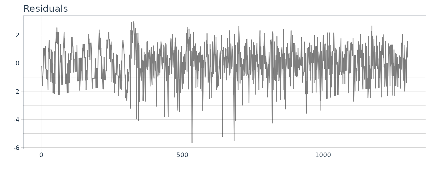
The residual plot for \(k=2\) shows a strong correlation and do not seem to be a white noise sequence.
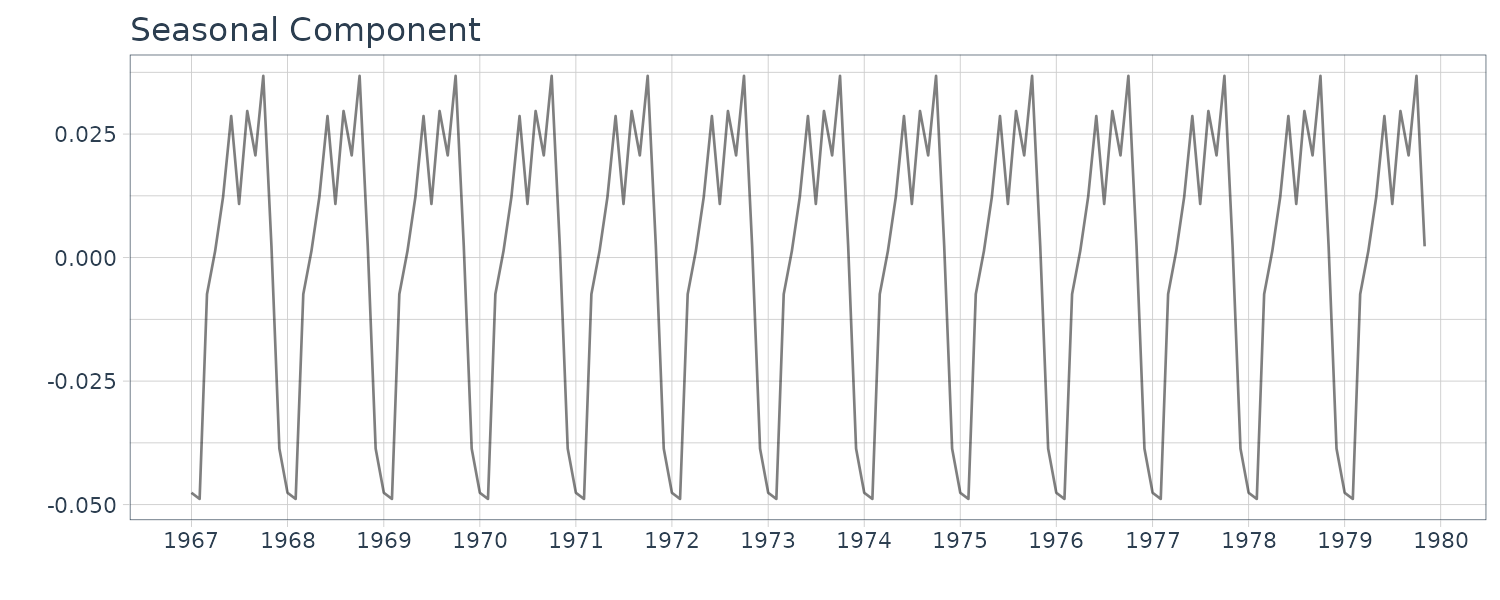
Seasonal Adjustment Model
In time series, a variable component \(s_{n}\) that repeats every year is called a seasonal component. In the following, p denotes the period length of the seasonal component. Here we put \(p = 12\) for monthly data and \(p = 4\) for quarterly data, respectively. Then, the seasonal component \(s_{n}\) approximately satisfies:
\[\begin{aligned} s_{n} &= s_{n-p} \end{aligned}\]Using the lag operator:
\[\begin{aligned} (1 - B^{p})s_{n} &= 0 \end{aligned}\]Similar to the stochastic trend component model introduced, a model for the seasonal component that gradually changes with time, is given by:
\[\begin{aligned} (1 - B^{p})^{l}s_{n} &= v_{n2} \end{aligned}\] \[\begin{aligned} v_{n2} &\sim N(0, \tau_{2}^{2}) \end{aligned}\]In particular, putting l = 1, we can obtain a random walk model for the seasonal component by:
\[\begin{aligned} s_{n} &= s_{n-p} + v_{n2} \end{aligned}\]In this model, it is assumed that \(s_{pn+i}\), \(n = 1, 2, \cdots\) is a random walk for any \(i = 1, \cdots , p\).
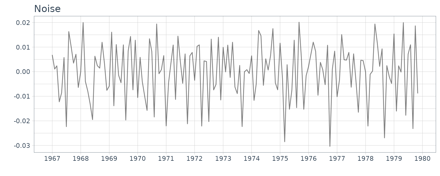
Therefore, assuming that the time series consists of the trend component \(t_{n}\), the seasonal component \(s_{n}\) and the observation noise \(w_{n}\), we obtain a basic model for seasonal adjustment as:
\[\begin{aligned} y_{n} &= t_{n} + s_{n} + w_{n} \end{aligned}\]However, the seasonal adjustment model:
\[\begin{aligned} (1 - B^{p})^{l}s_{n} &= v_{n2} \end{aligned}\]Would not work well in practice, because the trend component model and the seasonal component model both contain the common factor:
\[\begin{aligned} (1 - B)^{q}, q \geq 1 \end{aligned}\]We can decompose \((1 - B^{p})^{l}\):
\[\begin{aligned} (1 - B^{p})^{l} = (1 - B)^{l}(1 + B + \cdots + B^{p-1})^{l} \end{aligned}\]As we can see, the decomposition share the same \((1-B)^{q}, q \geq 1\) as the trend component.
Here, assume that \(e_{n}\) is an arbitrary solution of the difference equation:
\[\begin{aligned} (1 - B)^{q}e_{n} &= 0 \end{aligned}\]For q = 1, \(e_{n}\) is an arbitrary constant. If we define new components:
\[\begin{aligned} t_{n}' &= t_{n} + e_{n}\\ s_{n}' &= s_{n} - e_{n} \end{aligned}\]Then they satisfy:
\[\begin{aligned} (1 - B)t_{n}' &= t_{n}' - t_{n-1}'\\ &= t_{n} + e_{n} - (t_{n-1} + e_{n-1})\\ &= \Delta t_{n} - (1 - B)e_{n}\\ &= (1 - B)t_{n} \end{aligned}\] \[\begin{aligned} (1 - B^{p})s_{n}' &= (1 - B)(1 + B + \cdots + b^{p-1})s_{n}'\\ &= (1 - B)(1 + B + \cdots + b^{p-1})(s_{n} - e_{n})\\ &= s_{n} - s_{n-p} - [(1 - B)(1 + B + \cdots + b^{p-1})e_{n}]\\ &= s_{n} - s_{n-p} - 0\\ &= (1 - B^{p})s_{n} \end{aligned}\] \[\begin{aligned} y_{n} &= t_{n}' + s_{n}' + w_{n}\\ &= t_{n} + e_{n} + s_{n} - e_{n} + w_{n}\\ &= t_{n} + s_{n} + w_{n} \end{aligned}\]Therefore, we have infinitely many ways to decompose the time series yielding the same noise inputs \(v_{n1}, v_{n2}, w_{n}\). Moreover, since the likelihood of the model corresponding to those decompositions is determined only by \(v_{n1}, v_{n2}, w_{n}\), it is impossible to discriminate between the goodness of the decompositions by the likelihood. Therefore, if you use component models with common elements, the uniqueness of the decomposition is lost.
A simple way to guarantee uniqueness of decomposition is to ensure that none of the component models share any common factors.
Since:
\[\begin{aligned} 1 − B^{p} &= (1 − B)(1 + B + \cdots + B^{p−1}) \end{aligned}\]The sufficient condition for \((1 − B^{p})^{l} = 0\) is
\[\begin{aligned} (1 + B + \cdots + B^{p−1})^{l} &= 0 \end{aligned}\]So we just need to ensure:
\[\begin{aligned} \sum_{i=0}^{p-1}B^{i}s_{n} \approx 0 \end{aligned}\]Therefore, we will use the following model as a stochastic model for a seasonal component that changes gradually with time:
\[\begin{aligned} \Big(\sum_{i=0}^{p-1}B^{i}\Big)^{l}s_{n} &= v_{n2} \end{aligned}\] \[\begin{aligned} v_{n2} &\sim N(0, \tau_{2}^{2}) \end{aligned}\]The above is called the seasonal component model.
To obtain a state-space representation of the seasonal component model, initially we expand the operator as follows:
\[\begin{aligned} \Big(\sum_{i=0}^{p-1}B^{i}\Big)^{l}s_{n} &= 1 - \sum_{i=1}^{l\times(p-1)}d_{i}B^{i} \end{aligned}\]For \(l = 1\):
\[\begin{aligned} d_{i} &= -1 \end{aligned}\] \[\begin{aligned} i = 1, \cdots, p-1 \end{aligned}\]For \(l=2\):
\[\begin{aligned} d_{i} &= -i-1\\ i &\leq p-1 \end{aligned}\] \[\begin{aligned} d_{i} = &i+1 - 2p\\ p \leq &i \leq 2(p-1) \end{aligned}\]Since the seasonal component model given in is formally a special case of an autoregressive model, the state-space representation of the seasonal component model can be given as:
\[\begin{aligned} \textbf{x}_{n} &= \begin{bmatrix} s_{n}\\ s_{n-1}\\ \vdots\\ s_{n-l\times(p-1) + 1} \end{bmatrix} \end{aligned}\] \[\begin{aligned} \textbf{F} &= \begin{bmatrix} d_{1} & d_{2} & \cdots & d_{l\times(p-1)}\\ 1 & & &\\ & \ddots & &\\ && 1& \end{bmatrix} \end{aligned}\] \[\begin{aligned} \textbf{G} &= \begin{bmatrix} 1\\ 0\\ \vdots\\ 0 \end{bmatrix} \end{aligned}\] \[\begin{aligned} \textbf{H} &= \begin{bmatrix} 1 & 0 & \cdots 0 \end{bmatrix} \end{aligned}\]Standard Seasonal Adjustment Model
For standard seasonal adjustment, the time series \(y_{n}\) is decomposed into the following three components:
\[\begin{aligned} y_{n} &= t_{n} + s_{n} + w_{n} \end{aligned}\]Combining the basic model with the trend component model and the seasonal component model, we obtain the following standard seasonal adjustment models:
Observation Model:
\[\begin{aligned} y_{n} &= t_{n} + s_{n} + w_{n} \end{aligned}\]Trend Component Model:
\[\begin{aligned} \Delta^{k}t_{n} &= v_{n1} \end{aligned}\]Seasonal Component Model:
\[\begin{aligned} \Big(\sum_{i=1}^{p-1}B^{i}\Big)^{l}s_{n} &= v_{n2} \end{aligned}\] \[\begin{aligned} w_{n} &\sim N(0, \sigma^{2})\\ v_{n1} &\sim N(0, \tau_{1}^{2})\\ v_{n2} &\sim N(0, \tau_{2}^{2}) \end{aligned}\]For a seasonal adjustment model with trend order k, period p and seasonal order l = 1, let the (k + p − 1) dimensional state vector be defined by:
\[\begin{aligned} \textbf{x}_{n} = \begin{bmatrix} t_{n}\\ \vdots\\ t_{n−k+1}\\ s_{n}\\ s_{n−1}\\ \vdots\\ s_{n− p + 2} \end{bmatrix} \end{aligned}\]And the 2-dimensional noise vector:
\[\begin{aligned} \textbf{v}_{n} &= \begin{bmatrix} v_{n1}\\ v_{n2} \end{bmatrix} \end{aligned}\] \[\begin{aligned} \textbf{F} &= \begin{bmatrix} \textbf{F}_{1} & \textbf{0}\\ \textbf{0} & \textbf{F}_{2} \end{bmatrix} \end{aligned}\] \[\begin{aligned} \textbf{G} &= \begin{bmatrix} \textbf{G}_{1} & \textbf{0}\\ \textbf{0} & \textbf{G}_{2} \end{bmatrix} \end{aligned}\] \[\begin{aligned} \textbf{H} &= \begin{bmatrix} \textbf{H}_{1} & \textbf{H}_{2} \end{bmatrix} \end{aligned}\]Where \(\textbf{F}_{1}\), \(\textbf{G}_{1}\), \(\textbf{H}_{1}\) are the matrices and vectors used for the state-space representation of the trend component model, and similarly, \(\textbf{F}_{2}\), \(\textbf{G}_{2}\), \(\textbf{H}_{2}\) are the matrices and vectors used for the representation of the seasonal component model.
Then the state-space representation of the seasonal adjustment model is obtained as:
\[\begin{aligned} \textbf{x}_{n} &= \textbf{F}\textbf{x}_{n-1} + \textbf{G}\textbf{v}_{n}\\ \textbf{y}_{n} &= \textbf{H}\textbf{x}_{n} + \textbf{w}_{n} \end{aligned}\]For instance, if \(k = 2, l = 1, p = 4\), then:
\[\begin{aligned} \textbf{F} &= \begin{bmatrix} 2 & -1 & & &\\ 1 & 0 & & &\\ & & -1 & -1& -1\\ & & 1 & &\\ &&&1& \end{bmatrix} \end{aligned}\] \[\begin{aligned} \textbf{G} &= \begin{bmatrix} 1 & 0\\ 0 & 0\\ 0 & 1\\ 0 & 0\\ 0 & 0 \end{bmatrix} \end{aligned}\] \[\begin{aligned} \textbf{H} &= \begin{bmatrix} 1 & 0 & 1 & 0 & 0 \end{bmatrix} \end{aligned}\]Example: Seasonal adjustment of WHARD data
R function season of TSSS package fits the seasonal adjustment model and obtains trend and seasonal components. Various standard seasonal adjustment model can be obtained by specifying the following optional arguments:
- trend.order: trend order (0, 1, 2 or 3).
- season.order: seasonal order (0, 1 or 2).
- period: If the tsp attribute of y is NULL, period length of one season is required.
- tau2.ini: initial estimate of variance of the system noise \(\tau^{2}\), not equal to 1.
- filter: a numerical vector of the form c(x1,x2) which gives start and end position of filtering.
- predict: the end position of prediction (>= x2).
- log: logical. If TRUE, the data y is log-transformed.
- minmax: lower and upper limits of observations.
- plot: logical. If TRUE (default), ‘trend’ and ‘seasonal’ are plotted.
Note that this seasonal adjustment method can handle not only the monthly data, but also verious period length. For example, set period = 4 for quarterly data, = 12 for monthly data, = 5 or 7 for weekly data and = 24 for hourly data.
The function season yields the following outputs:
- tau2: variance of the system noise.
- sigma2: variance of the observational noise.
- llkhood: log-likelihood of the model.
- aic: AIC of the model.
- trend: trend component (for trend.order > 0).
- seasonal: seasonal component (for seasonal.order > 0).
- noise: noise component.
- cov: covariance matrix of smoother.
dat <- as.ts(
  WHARD |>
    select(value)
)

fit <- season(
  dat,
  trend.order = 2,
  seasonal.order = 1,
  log = TRUE,
  log.base = 10
)

> fit
 tau2		 2.59416e-02	 1.09998e-08
 sigma2		 1.50164e-04
 log-likelihood	     342.532
 aic		    -655.065

> names(fit)
 [1] "tau2"       "sigma2"     "llkhood"    "aic"        "trend"
 [6] "seasonal"   "arcoef"     "ar"         "day.effect" "noise"
[11] "cov"
The maximum likelihood estimates of the parameters are:
\[\begin{aligned} \hat{\tau}_{1}^{2} &= 0.0259\\ \hat{\tau}_{2}^{2} &= 0.0110 \times 10^{-7}\\ \hat{\sigma}^{2} &= 0.150 \times 10^{-3}\\ \text{AIC} &= -655 \end{aligned}\]WHARD <- WHARD |>
mutate(
trend = fit$trend,
seasonal = fit$seasonal,
sd = sqrt(fit$cov * fit$sigma2),
noise = fit$noise$val |>
as.numeric()
)
The function season can also perform long-term prediction based on the estimated seasonal adjustment model. For that purpose, use the argument filter to specify the data period to be used for the estimation of the parameters. In the example below, filter = c(1, 132) indicates that the seasonal adjustment model is estimated from the data \(y_{1}, \cdots, y_{132}\) and the rest of the data \(y_{133}, \cdots, y_{N}\) are predicted based on the estimated model.
fit2 <- season(
  dat,
  trend.order = 2,
  seasonal.order = 1,
  filter = c(1, 132),
  log = TRUE,
  log.base = 10
)

WHARD <- WHARD |>
  mutate(
    trend = fit2$trend,
    seasonal = fit2$seasonal,
    sd = sqrt(fit2$cov * fit2$sigma2)
  )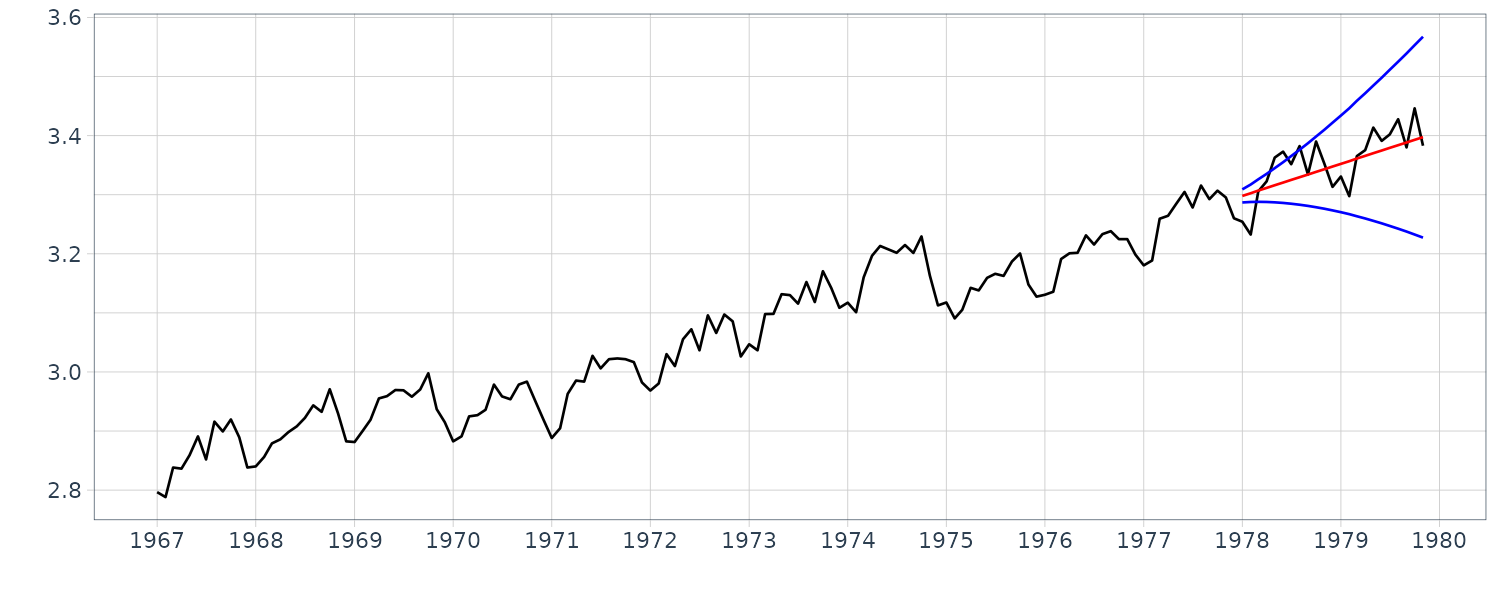
In the figure, the mean of the predictive distribution \(y_{132+ j\mid 132}\) and the \(\pm 1\) standard error interval, i.e., \(\pm d_{132+ j\mid 132}\) for \(j = 1, \cdots, 24\) are shown. The actual observations are also shown. In this case, very good long-term prediction can be attained, because the estimated trend and seasonal components are steady. However, it should be noted that ±1 standard error interval is very wide indicating that the long-term prediction by this model is not so reliable.
Decomposition Including a Stationary AR Component
In this section, we consider an extension of the standard seasonal adjustment method. In the standard seasonal adjustment method, the time series is decomposed into three components, i.e. the trend component, the seasonal component and the observation noise. These components are assumed to follow the models:
\[\begin{aligned} y_{n} &= t_{n} + s_{n} + w_{n} \end{aligned}\] \[\begin{aligned} \Delta^{k}t_{n} &= v_{n1} \end{aligned}\] \[\begin{aligned} \Big(\sum_{i=1}^{p-1}B^{i}\Big)^{l}s_{n} &= v_{n2} \end{aligned}\]And the observation noise is assumed to be a white noise. Therefore, if a significant deviation from that assumption is present, then the decomposition obtained by the standard seasonal adjustment method might become inappropriate.
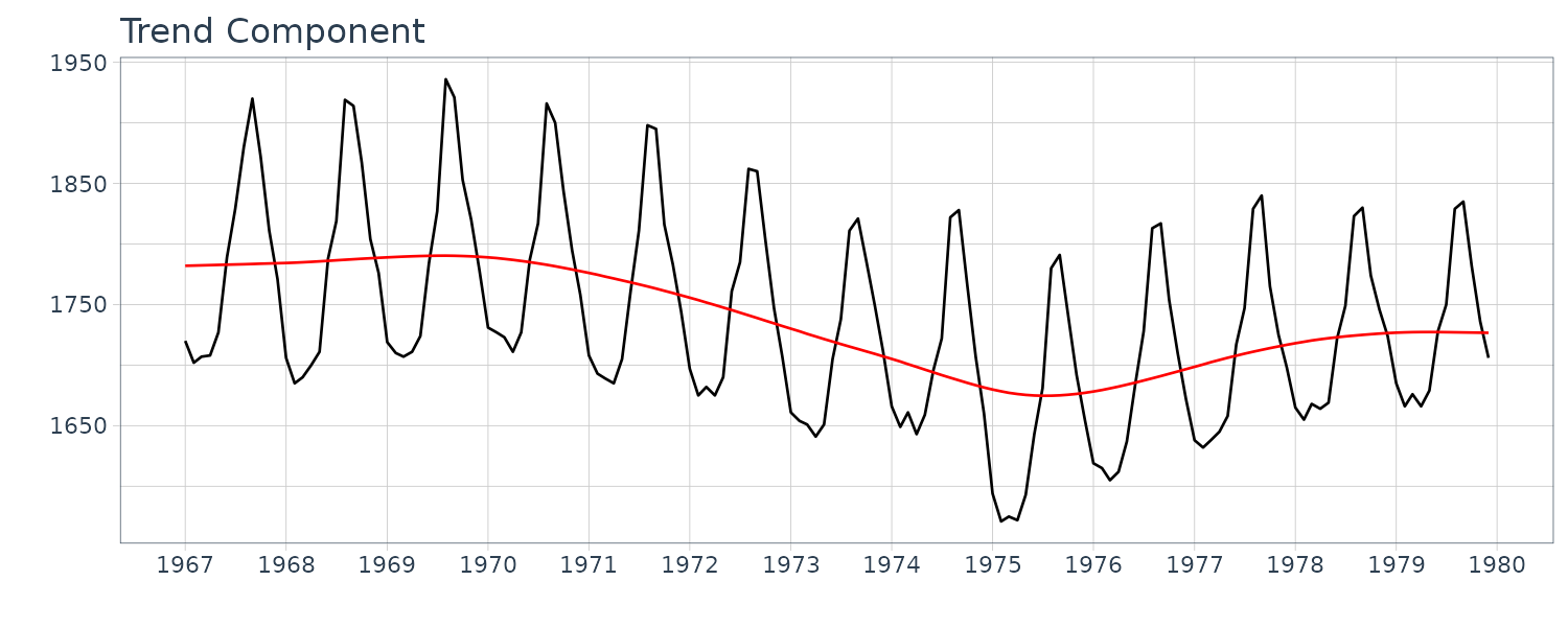
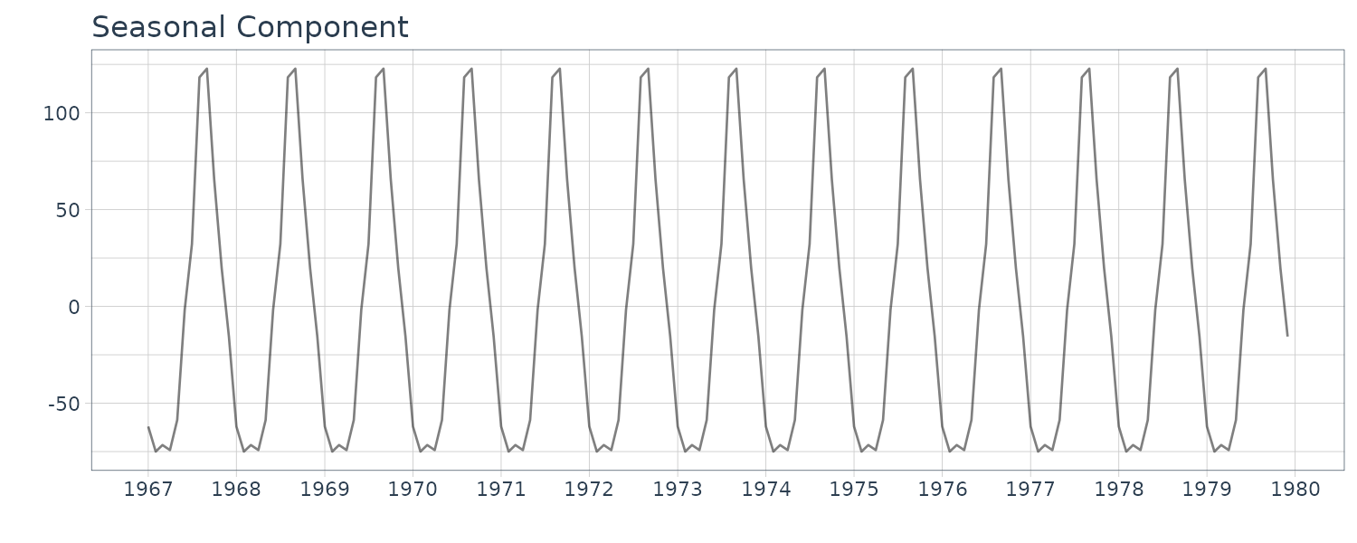
Running the standard seasonal adjustment method for the model with k = 2, l = 1 and p = 12 on the BLSALLFOOD dataset. In this case, different from the case shown in the previous section, the estimated trend shows a wiggle, particularly in the latter part of the data.
dat <- as.ts(
  BLSALLFOOD |>
    select(value)
)

fit <- season(
  dat,
  trend.order = 2,
  seasonal.order = 1
)
names(fit)

BLSALLFOOD <- BLSALLFOOD |>
  mutate(
    trend = fit$trend,
    seasonal = fit$seasonal
  )
Running the long-term prediction on the dataset with a 2-year prediction horizon:
fit <- season(
  dat,
  trend.order = 2,
  seasonal.order = 1,
  filter = c(1, 132)
)

BLSALLFOOD <- BLSALLFOOD |>
  mutate(
    trend = fit$trend,
    seasonal = fit$seasonal,
    sd = sqrt(fit$cov * fit$sigma2)
  )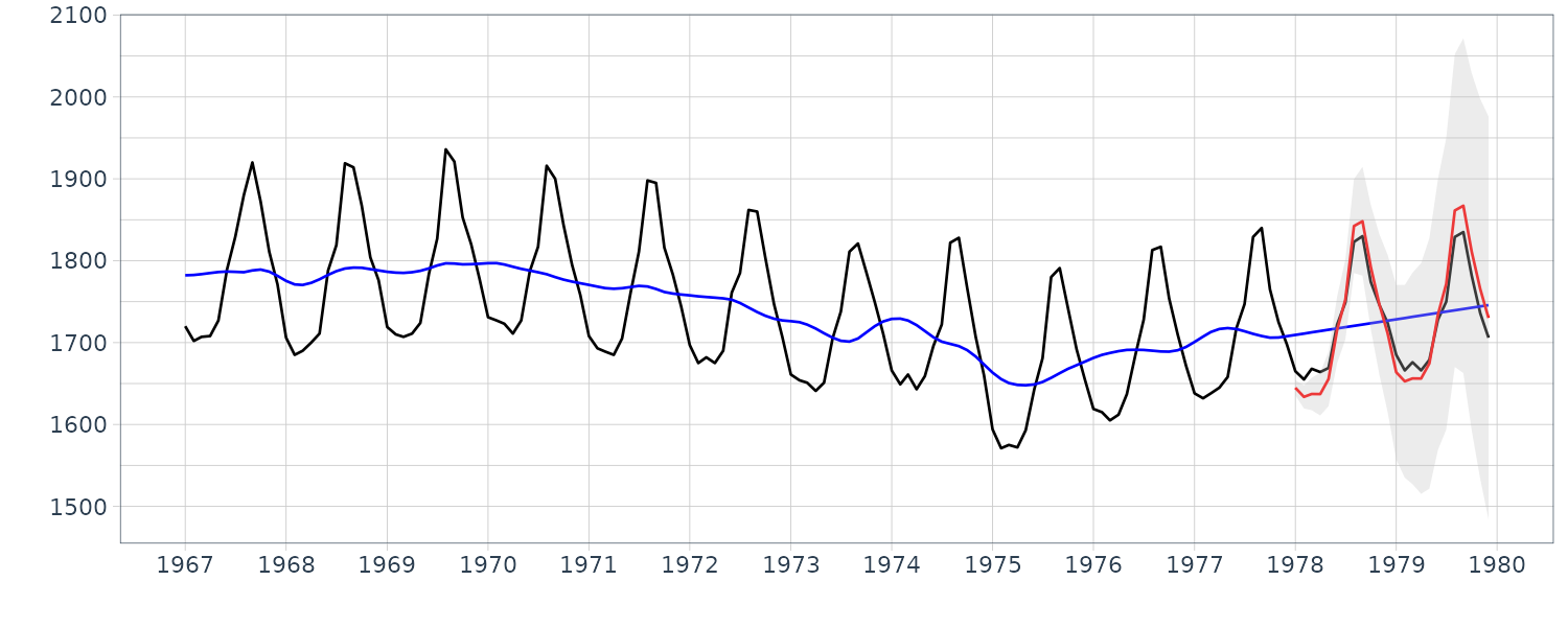
In this case, apparently the predicted mean \(y_{132+ j\mid 132}\) provides a reasonable prediction of the actual time series \(y_{132+ j}\). However it is evident that prediction by this model is not reliable, because an explosive increase of the width of the confidence interval is observed.
The long-term predictions starting at and before n = 130 have significant downward bias. On the other hand, the long-term predictions starting at and after n = 135 have significant upward bias. This is the reason that the explosive increase in the width of the confidence interval has occurred when the lead time has increased in the long-term predictions.
The stochastic trend component model in the seasonal adjustment model can flexibly express a complex trend component. But in the long-term prediction with this model, the predicted mean \(t_{n+ j\mid n}\) is simply obtained by using the difference equation
\[\begin{aligned} \Delta^{k}t_{n+j| n} = 0 \end{aligned}\]Therefore, whether the predicted values go up or down is decided by the starting point of the trend. From these results, we see that if the estimated trend is wiggly, it is not appropriate to use the standard seasonal adjustment model for long-term prediction.
In predicting one year or two years ahead (12 or 24 values), it is possible to obtain a better prediction with a smoother curve by using a smaller value than the maximum likelihood estimate for the system noise variance of the trend component, \(\tau_{1}^{2}\). However, this method suffers from the following problems; it is difficult to reasonably determine \(\tau_{1}^{2}\) and, moreover, prediction with a small lead time such as one-step-ahead prediction becomes significantly worse than that obtained by the maximum likelihood model.
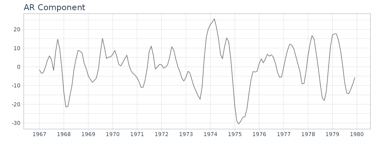
To achieve good prediction for both short and long lead times, we consider an extension of the standard seasonal adjustment model by including a new component \(p_{n}\) as:
\[\begin{aligned} y_{n} &= t_{n} + s_{n} + p_{n} + w_{n} \end{aligned}\]Here \(p_{n}\) is a stationary AR component model that is assumed to follow an AR model:
\[\begin{aligned} p_{n} &= \sum_{i=1}^{m_{3}}a_{i}p_{n-i} + v_{n3} \end{aligned}\] \[\begin{aligned} v_{n3} &\sim N(0, \tau_{3}^{2}) \end{aligned}\]This model expresses a short-term variation such as the cycle of an economic time series, not a long-term tendency like the trend component. In the model, the trend component obtained by the standard seasonal adjustment model is further decomposed into the smoother trend component \(t_{n}\) and the short-term variation \(p_{n}\).
The state-space representation:
\[\begin{aligned} \textbf{x}_{n} &= \begin{bmatrix} p_{n}\\ p_{n-1}\\ \vdots\\ p_{n-m3 + 1} \end{bmatrix} \end{aligned}\] \[\begin{aligned} \textbf{F}_{3} &= \begin{bmatrix} a_{1} & a_{2} & \cdots & a_{m3}\\ 1 & & &\\ & \ddots & &\\ &&1& \end{bmatrix} \end{aligned}\] \[\begin{aligned} \textbf{G}_{3} &= \begin{bmatrix} 1\\ 0\\ \vdots\\ 0 \end{bmatrix} \end{aligned}\] \[\begin{aligned} \textbf{H}_{3} &= \begin{bmatrix} 1 & 0 & \cdots & 0 \end{bmatrix} \end{aligned}\] \[\begin{aligned} \textbf{Q}_{3} &= \boldsymbol{\tau}_{3}^{2} \end{aligned}\]Therefore, using the state-space representation for the composite model, the state-space model for the decomposition:
\[\begin{aligned} \textbf{F} &= \begin{bmatrix} \textbf{F}_{1} & &\\ & \textbf{F}_{2} &\\ &&\textbf{F}_{3} \end{bmatrix} \end{aligned}\] \[\begin{aligned} \textbf{G} &= \begin{bmatrix} \textbf{G}_{1} & &\\ & \textbf{G}_{2} &\\ &&\textbf{G}_{3} \end{bmatrix} \end{aligned}\] \[\begin{aligned} \textbf{H} &= \begin{bmatrix} \textbf{H}_{1} & \textbf{H}_{2} & \textbf{H}_{3} \end{bmatrix} \end{aligned}\] \[\begin{aligned} \textbf{Q} &= \begin{bmatrix} \boldsymbol{\tau}_{1}^{2} & &\\ & \boldsymbol{\tau}_{2}^{2} &\\ & &\boldsymbol{\tau}_{3}^{2} \end{bmatrix} \end{aligned}\]Example: Seasonal adjustment with stationary AR component
To fit a seasonal adjustment model including an AR component by the function season, it is only necessary to specify the AR order by the ar.order parameter as follows:
fit <- season(
  dat,
  trend.order = 2,
  seasonal.order = 1,
  ar.order = 2
)
fit
names(fit)

BLSALLFOOD <- BLSALLFOOD |>
  mutate(
    trend = fit$trend,
    seasonal = fit$seasonal,
    ar = fit$ar
  )
The following good prediction was achieved for both short and long lead times with this modeling:
fit <- season(
  dat,
  trend.order = 2,
  seasonal.order = 1,
  ar.order = 2,
  filter = c(1, 132)
)

BLSALLFOOD <- BLSALLFOOD |>
  mutate(
    trend = fit$trend,
    seasonal = fit$seasonal,
    ar = fit$ar,
    sd = sqrt(fit$cov * fit$sigma2)
  )
Decomposition Including a Trading-Day Effect
Monthly economic time series, such as the amount of sales at a department store, may strongly depend on the number of the days of the week in each month, because there are marked differences in sales depending on the days of the week. For example, a department store would have more customers on Saturdays and Sundays or may regularly close on a specific day of the week. A similar phenomenon can often be seen in environmental data, for example, the daily amounts of NOx and CO2.
A trading-day adjustment has been developed to remove such trading-day effects that depend on the number of the days of the week. Hereafter, the number of Sundays to Saturdays in the n-th month, \(y_{n}\), are denoted as:
\[\begin{aligned} d_{n1}^{*}, \cdots, d_{n7}^{*} \end{aligned}\]Note that each \(d_{ni}^{*}\) takes a value 4 or 5 for monthly data.
Then the effect of the trading-day is expressed as:
\[\begin{aligned} \text{td}_{n} &= \sum_{i=1}^{7}\beta_{ni}d_{ni}^{*} \end{aligned}\]The coefficient \(\beta_{ni}\) expresses the effect of the number of the i-th day of the week on the value of \(y_{n}\). Here, to guarantee the uniqueness of the decomposition of the time series, we impose the restriction that the sum of all coefficients amounts to 0, that is:
\[\begin{aligned} \beta_{n1} + \cdots + \beta_{n7} &= 0 \end{aligned}\]Then, since the last coefficient is defined by:
\[\begin{aligned} \beta_{n7} = −(\beta_{n1} + \cdots + \beta_{n6}) \end{aligned}\]Then the trading-day effect can be expressed by:
\[\begin{aligned} \text{td}_{n} &= \sum_{i=1}^{6}\beta_{ni}(d_{ni}^{*} - d_{n7}^{*})\\ &= \sum_{i}^{6}\beta_{ni}d_{ni} \end{aligned}\]Where:
\[\begin{aligned} d_{ni} &= d_{ni}^{*} - d_{n7}^{*} \end{aligned}\]Is the difference in the number of the i-th day of the week and the number of Saturdays in the n-th month, \(y_{n}\).
This is so as:
\[\begin{aligned} \sum_{i=1}^{7}\beta_{ni}d_{ni}^{*} &= \sum_{i=1}^{6}\beta_{ni}d_{ni}^{*} + \beta_{n7}d_{n7}^{*}\\ &= \sum_{i=1}^{6}\beta_{ni}d_{ni}^{*} - (\beta_{n1} + \cdots + \beta_{n6})d_{n7}^{*}\\ &= \sum_{i}^{6}\beta_{ni}d_{ni} \end{aligned}\]On the assumption that these coefficients gradually change, following the first order trend model:
\[\begin{aligned} \Delta \beta_{ni} &= v_{n4}^{(i)}\\ v_{n4}^{(i)} &\sim N(0, \tau_{4}^{2}) \end{aligned}\] \[\begin{aligned} i = 1, \cdots, 6 \end{aligned}\]The state-space representation of the trading-day effect model is obtained by:
\[\begin{aligned} \textbf{x}_{n4} &= \begin{bmatrix} \beta_{n1}\\ \vdots\\ \beta_{n6} \end{bmatrix} \end{aligned}\] \[\begin{aligned} \textbf{F}_{n4} &= \textbf{G}_{n4} = \textbf{I}_{6} \end{aligned}\] \[\begin{aligned} \textbf{H}_{n4} &= \begin{bmatrix} d_{n1} & \cdots & d_{n6} \end{bmatrix} \end{aligned}\] \[\begin{aligned} \textbf{Q} &= \begin{bmatrix} \tau_{4}^{2} & &\\ & \ddots &\\ && \tau_{4}^{2} \end{bmatrix} \end{aligned}\]In this representation, \(\textbf{H}_{n4}\) becomes a time-dependent vector. For simplicity, the covariance matrix \(\textbf{Q}\) is assumed to be a diagonal matrix with equal diagonal elements.
In actual analysis, however, we often assume that the coefficients are time-invariant:
\[\begin{aligned} \beta_{ni} &= \beta_{i} \end{aligned}\]Which can be implemented by putting either \(\tau_{4}^{2} = 0\) or \(\textbf{G} = \textbf{0}\) in the state-space representation of the model.
The state-space model for the decomposition of the time series:
\[\begin{aligned} y_{n} &= t_{n} + s_{n} + p_{n} + \text{td}_{n} + w_{n} \end{aligned}\]Is obtained by using:
\[\begin{aligned} \textbf{x}_{n} &= \begin{bmatrix} \textbf{x}_{n1}\\ \textbf{x}_{n2}\\ \textbf{x}_{n3}\\ \textbf{x}_{n4} \end{bmatrix} \end{aligned}\] \[\begin{aligned} \textbf{F} &= \begin{bmatrix} \textbf{F}_{1} & & &\\ & \textbf{F}_{2} & &\\ & & \textbf{F}_{3} &\\ & & &\textbf{F}_{4} \end{bmatrix} \end{aligned}\] \[\begin{aligned} \textbf{G} &= \begin{bmatrix} G_{1} & &\\ & G_{2} &\\ & & G_{3}\\ 0 & 0 & 0 \end{bmatrix} \end{aligned}\] \[\begin{aligned} \textbf{H} &= \begin{bmatrix} \textbf{H}_{1} & \textbf{H}_{2} & \textbf{H}_{3} & \textbf{H}_{4} \end{bmatrix} \end{aligned}\] \[\begin{aligned} \textbf{Q} &= \begin{bmatrix} \tau_{1}^{2} & &\\ & \tau_{2}^{2} &\\ & & \tau_{3}^{2} \end{bmatrix} \end{aligned}\]Example: Seasonal adjustment with trading-day effect
fit <- season(
  dat,
  trend.order = 2,
  seasonal.order = 1,
  ar.order = 0,
  trade = TRUE,
  log = TRUE,
  log.base = 10
)

> fit
 tau2		 1.26964e-01	 1.09998e-08
 sigma2		 5.77411e-05
 log-likelihood	     358.232
 aic		    -674.464

> names(fit)
 [1]  "tau2"      "sigma2"  "llkhood"  "aic"        "trend"
 [6]  "seasonal"  "arcoef"  "ar"       "day.effect" "noise"
 [11] "cov"

WHARD <- WHARD |>
  mutate(
    trend = fit$trend,
    seasonal = fit$seasonal,
    day.effect = fit$day.effect,
    ar = fit$ar
  )
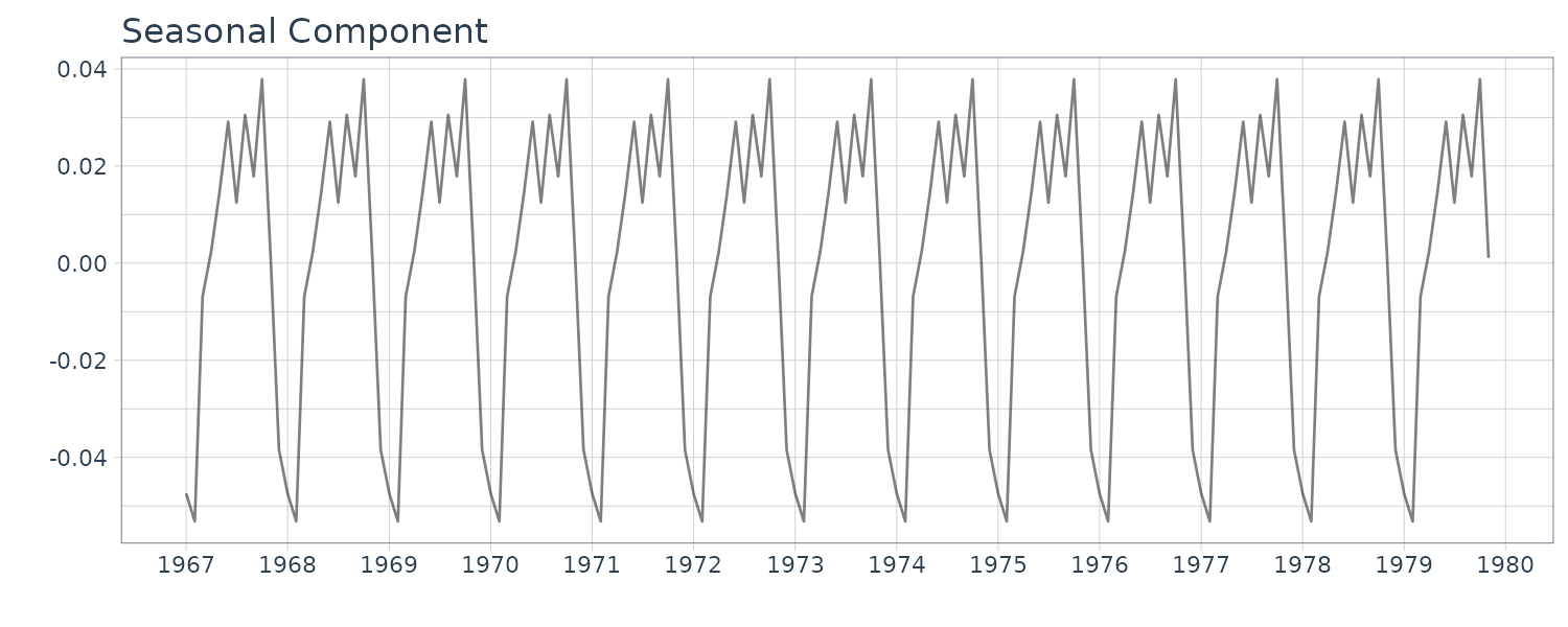

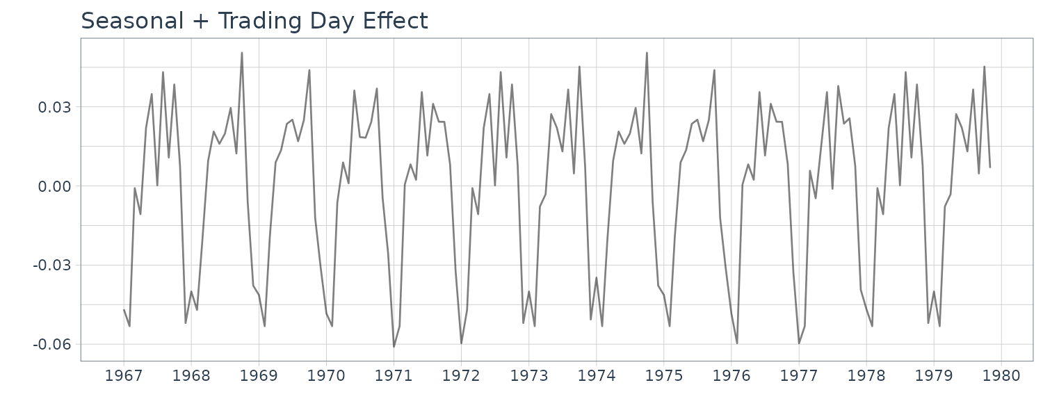
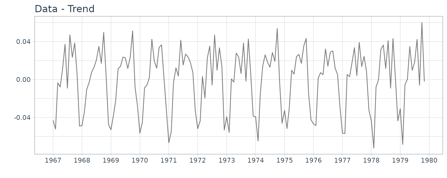
Although the extracted trading-day effect component is apparently minuscule, it can be seen that the plot of seasonal component plus trading-day effect component reproduces the details of the observed time series. The AIC value for this model is −778.18 which is significantly smaller than that for the standard seasonal adjustment model, −728.50.
Once the time-invariant coefficients of trading-day effects \(\beta_{i}\) are estimated, this can contribute to a significant increase in the accuracy of prediction, because \(d_{n1}, \cdots, d_{n6}\) are known even for the future.
Although the trading-day effect is minuscule, the seasonal component plus trading-day effect is quite similar to the data minus trend component. This suggests that a considerable part of the noise component of the standard seasonal adjustment model can be expressed as the trading-day effect:
Time-Varying Variance Model
Example: Time-varying variance of a seismic data
The time series \(y_{n}\), \(n = 1, \cdots, N\), is assumed to be a Gaussian white noise with mean 0 and time-varying variance \(\sigma_{n}^{2}\).
Assuming that:
\[\begin{aligned} \sigma_{2m-1}^{2} &= \sigma_{2m}^{2} \end{aligned}\]If we define a transformed series \(s_{1}, \cdots, s_{\frac{N}{2}}\):
\[\begin{aligned} s_{m} &= y_{2m-1}^{2} + y_{2m}^{2} \end{aligned}\]\(s_{m}\) is distributed a \(\chi^{2}\)-distribution with \(\text{df} = 2\), which is known to be an exponential distribution.
The exponential distribution of \(s_{m}\) is given by:
\[\begin{aligned} f(s) &= \frac{1}{2\sigma^{2}}e^{-\frac{s}{2\sigma^{2}}} \end{aligned}\]The probability density function of the random variable \(z_{m}\) defined by the transformation:
\[\begin{aligned} z_{m} &= \log\frac{s_{m}}{2} \end{aligned}\]Is expressed as:
\[\begin{aligned} g(z) &= \frac{1}{\sigma^{2}}e^{z-\frac{e^{z}}{\sigma^{2}}}\\ &= e^{(z - \log \sigma^{2}) - e^{(z - \log \sigma^{2})}} \end{aligned}\]This means that the transformed series \(z_{m}\) can be written as:
\[\begin{aligned} z_{m} &= \log \sigma_{m}^{2} + w_{m} \end{aligned}\]Where \(w_{m}\) follows a double exponential distribution with pdf:
\[\begin{aligned} h(w) &= e^{w - e^{w}} \end{aligned}\]Therefore, assuming that the logarithm of the time-varying variance, \(\log \sigma_{m}^{2}\), follows a k-th order trend component model, the transformed series \(z_{m}\) can be expressed by a state-space model:
\[\begin{aligned} \Delta^{k}t_{m} &= v_{m} \end{aligned}\] \[\begin{aligned} z_{m} &= t_{m} + w_{m} \end{aligned}\]It should be noted that the distribution of the noise \(w_{m}\) is not Gaussian. However, since the mean and the variance of the double exponential distribution are given by \(−\xi = 0.57722\) (Euler constant) and \(\frac{\pi^{2}}{6}\), respectively, we can approximate it by a Gaussian distribution as follows:
\[\begin{aligned} w_{m} &\sim N(-\xi, \frac{\pi^{2}}{6}) \end{aligned}\]So far, the transformed series defined as the mean of two consecutive squared time series has been used in estimating the variance of the time series. This is just to make the noise distribution \(g(z)\) closer to a Gaussian distribution, and it is not essential in estimating the variance of the time series. In fact, if we use a non-Gaussian filter for trend estimation, we can use the transformed series \(s_{n} = y_{n}^{2}\), \(n = 1, \cdots, N\), and with this transformation, it is not necessary to assume that \(\sigma_{2m−1} = \sigma_{2m}\).
R function tvvar of the package TSSS estimates time-varying variance.
The input arguments:
- trend.order: specifies the order of the trend component model
- tau2.ini and delta, respectively, specify the initial estimate of the variance of the system noise \(\tau^{2}\) and the search width for finding the maximum likelihood estimate. If they are not given explicitly, i.e. if tau2.ini = NULL, the most suitable value is chosen within the candidates \(\tau^{2} = 2^{-k}, k = 1, 2, \cdots\).
Then the function tvvar returns the following outputs:
- tvv: time-varying variance
- nordata: normalized data
- sm: transformed data
- trend: trend of the transformed data sm
- noise: residuals
- tau2: variance of the system noise
- sigma2: variance of the observation noise
- llkhood: log-likelihood of the model
- aic: AIC of the model
- tsname: the name of the time series yn
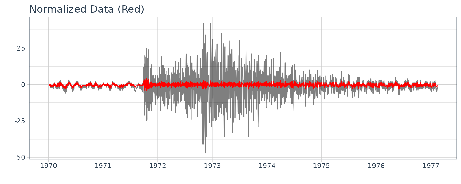
The function tvvar was applied to the MYE1F seismic data shown below using trend order 2 and the initial variance \(\tau^{2} = 0.66 \times 10^{−5}\). The plots below show the transformed data \(s_{m}\), the estimates of the logarithm of the variance \(\log \hat{\sigma}_{m}^{2}\), the residual \(s_{m} − \log \hat{\sigma}_{m}^{2}\) and the normalized time series obtained by: \(\begin{aligned} \tilde{y}_{n} = \frac{y_{n}}{\hat{\sigma}_{\frac{n}{2}}} \end{aligned}\)
By this normalization, we can obtain a time series with a variance roughly equal to 1.
dat <- as.ts(MYE1F)

fit <- tvvar(
  dat,
  trend.order = 2,
  tau2.ini = 6.6e-06,
  delta = 1.0e-06
)

> fit
 tau2		 6.60000e-06
 sigma2		 9.71228e-01
 log-likelihood	   -2195.731
 aic		    4399.462

> names(fit)
[1] "tvv"  "nordata" "sm"      "trend"  "noise"
[6] "tau2" "sigma2"  "llkhood" "aic"    "tsname"

dat <- tsibble(
  t = 1:length(fit$tvv),
  tvv = fit$tvv,
  sm = fit$sm,
  trend = fit$trend[, 2],
  upper = fit$trend[, 3],
  lower = fit$trend[, 1],
  noise = fit$noise,
  index = t
)
Time-Varying Coefficient AR Model
The characteristics of stationary time series can be expressed by an autocovariance function or a power spectrum. Therefore, for nonstationary time series with a time-varying stochastic structure, it is natural to consider that its autocovariance function and power spectrum change over time.
An autoregressive model with time-varying coefficients for the nonstationary time series \(y_{n}\) is modeled as:
\[\begin{aligned} y_{n} &= \sum_{j=1}^{m}a_{nj}y_{n-j} + w_{n} \end{aligned}\] \[\begin{aligned} w_{n} &\sim N(0, \sigma^{2}) \end{aligned}\]This model is called the time-varying coefficients AR model of order \(m\) and \(a_{nj}\) is called the time-varying AR coefficient with time lag \(j\) at time \(n\). Given the time series \(y_{1}, \cdots, y_{N}\), this time-varying coefficients AR model contains at least \(m\times N\) unknown coefficients. The difficulty with this type of model is, therefore, that we cannot obtain meaningful estimates by applying the ordinary maximum likelihood method or the least squares method.
To circumvent this difficulty, similar to the cases of the trend model and the seasonal adjustment model, we use a stochastic trend component model to represent time-varying parameters of the AR model.
In the case of the trend model, we considered the trend component \(t_{n}\) as an unknown parameter and introduced the model for its time change. Similarly, in the case of a time-varying coefficent AR model, since the AR coefficient \(a_{nj}\) changes over time \(n\), we consider a constraint model:
\[\begin{aligned} \Delta^{k}a_{nj} &= v_{nj} \end{aligned}\] \[\begin{aligned} j &= 1, \cdots, m \end{aligned}\]The vector:
\[\begin{aligned} \textbf{v}_{n} &= \begin{bmatrix} v_{n1}\\ \vdots\\ v_{nm} \end{bmatrix} \end{aligned}\]is an m-dimensional Gaussian white noise with mean vector \(\textbf{0}\) and covariance matrix \(\textbf{Q}\). Since \(v_{ni}\) and \(v_{nj}\) are usually assumed to be independent for \(i \neq j\):
\[\begin{aligned} \textbf{Q} &= \begin{bmatrix} \tau_{11}^{2} & &\\ & \ddots &\\ & & \tau_{mm}^{2} \end{bmatrix} \end{aligned}\]It is further assumed that:
\[\begin{aligned} \tau_{11}^{2} &= \cdots = \tau_{mm}^{2} = \tau^{2} \end{aligned}\]The rationale for this assumption will be discussed later.
The state-space representation:
For k = 1:
\[\begin{aligned} x_{nj}^{(1)} &= a_{nj} \end{aligned}\] \[\begin{aligned} F^{(1)} &= G^{(1)} = 1 \end{aligned}\]For k = 2:
\[\begin{aligned} \textbf{x}_{nj}^{(2)} &= \begin{bmatrix} a_{nj}\\ a_{n-1, j} \end{bmatrix} \end{aligned}\] \[\begin{aligned} \textbf{F}^{(2)} &= \begin{bmatrix} 2 & -1\\ 1 & 0 \end{bmatrix} \end{aligned}\] \[\begin{aligned} \textbf{G}^{(2)} &= \begin{bmatrix} 1\\ 0 \end{bmatrix} \end{aligned}\]Assuming the j-th term of equation to be the j-th component of this model, it can be expressed as:
\[\begin{aligned} H_{n}^{(1j)} &= y_{n-j}\\ \textbf{H}_{n}^{(2j)} &= \begin{bmatrix} y_{n-j}\\ 0 \end{bmatrix} \end{aligned}\]Noting that:
\[\begin{aligned} H^{(1)} &= 1\\ \textbf{H}^{(2)} &= \begin{bmatrix} 1\\ 0 \end{bmatrix}\\ \textbf{H}_{n}^{(kj)} &= y_{n-j}\textbf{H}^{(k)} \end{aligned}\]Then the j-th component of the time-varying coefficient AR model is given by a state-space model:
\[\begin{aligned} \textbf{x}_{nj} &= \textbf{F}^{(k)}\textbf{x}_{n-1,j} + \textbf{G}^{(k)}\textbf{v}_{nj} \end{aligned}\] \[\begin{aligned} a_{nj}y_{n-j} &= \textbf{H}_{n}^{(kj)}\textbf{x}_{nj} \end{aligned}\]Using the above component models, a state-space representation of the time-varying coefficients AR model is obtained as:
\[\begin{aligned} \textbf{x}_{n} &= \textbf{F}\textbf{x}_{n-1} + \textbf{Gv}_{n}\\ y_{n} &= \textbf{H}_{n}\textbf{x}_{n} + w_{n} \end{aligned}\]Where the \(km \times km\) matrix \(\textbf{F}\), the \(km \times m\) matrix \(\textbf{G}\) and the \(km\)-dimensional vectors \(\textbf{H}_{n}\) and \(\textbf{x}_{n}\) are defined by:
\[\begin{aligned} \textbf{F} &= \begin{bmatrix} \mathbf{F}^{(k)} & &\\ & \ddots &\\ & & \mathbf{F}^{(k)} \end{bmatrix}\\ &= \textbf{I}_{m} \otimes \textbf{F}^{(k)} \end{aligned}\] \[\begin{aligned} \textbf{G} &= \begin{bmatrix} \mathbf{G}^{(k)} & &\\ & \ddots &\\ & & \mathbf{G}^{(k)} \end{bmatrix}\\ &= \textbf{I}_{m} \otimes \textbf{G}^{(k)} \end{aligned}\] \[\begin{aligned} \textbf{H}_{n} &= \begin{bmatrix} \textbf{H}_{n}^{(k1)}\\ \cdots\\ \textbf{H}_{n}^{(km)} \end{bmatrix}\\ &= \begin{bmatrix} y_{n-1}\\ \vdots\\ y_{n-m} \end{bmatrix} \otimes \mathbf{H}^{(k)} \end{aligned}\] \[\begin{aligned} \textbf{x}_{n} &= \begin{cases} \begin{bmatrix} a_{n1}\\ \vdots\\ a_{nm} \end{bmatrix} & k = 1\\[5pt] \begin{bmatrix} a_{n1}\\ a_{n-1, 1}\\ \vdots\\ a_{nm}\\ a_{n-1, m} \end{bmatrix} & k=2 \end{cases} \end{aligned}\] \[\begin{aligned} \textbf{Q} &= \begin{bmatrix} \tau^{2} & &\\ & \tau^{2} &\\ & & \tau^{2} \end{bmatrix} \end{aligned}\] \[\begin{aligned} R &= \sigma^{2} \end{aligned}\]For instance, for \(m = 2\) and \(k = 2\), the state-space model is defined as:
\[\begin{aligned} \begin{bmatrix} a_{n1}\\ a_{n-1, 1}\\ a_{n2}\\ a_{n-1, 2} \end{bmatrix} &= \begin{bmatrix} 2 & -1 & 0 & 0\\ 1 & 0 & 0 & 0\\ 0 & 0 & 2 & -1\\ 0 & 0 & 1 & 0 \end{bmatrix} \begin{bmatrix} a_{n-1,1}\\ a_{n-2, 1}\\ a_{n-1, 2}\\ a_{n-2, 2} \end{bmatrix} + \begin{bmatrix} 1 & 0\\ 0 & 0\\ 0 & 1\\ 0 & 0 \end{bmatrix} \begin{bmatrix} v_{n1}\\ v_{n2} \end{bmatrix} \end{aligned}\] \[\begin{aligned} y_{n} &= \begin{bmatrix} y_{n-1} & 0 & y_{n-2} & 0 \end{bmatrix} \begin{bmatrix} a_{n1}\\ a_{n-1, 1}\\ a_{n2}\\ a_{n-1, 2} \end{bmatrix} + w_{n} \end{aligned}\] \[\begin{aligned} \begin{bmatrix} v_{n, 1}\\ v_{n, 2} \end{bmatrix} &\sim N\Bigg( \begin{bmatrix} 0\\ 0 \end{bmatrix}, \begin{bmatrix} \tau^{2} & 0\\ 0 & \tau^{2} \end{bmatrix} \Bigg) \end{aligned}\] \[\begin{aligned} w_{n} &\sim N(0, \sigma^{2}) \end{aligned}\]The variance \(\sigma^{2}\) of the observation noise \(w_{n}\) and the variance \(\tau^{2}\) of the system noise \(\textbf{v}_{n}\) can be estimated by the maximum likelihood method.
The AR order \(m\) and the order \(k\) of the smoothness constraint model can be determined by minimizing the information criterion AIC. Given the orders \(m\) and \(k\) and the estimated variances \(\hat{\sigma}^{2}, \hat{\tau}^{2}\), the smoothed estimate of the state vector \(\textbf{x}_{n\mid N}\) is obtained by the fixed interval smoothing algorithm. Then the \([(j − 1)k + 1]\)-th element of the estimated state gives the smoothed estimate of the time-varying AR coefficient \(\hat{a}_{n, j\mid N}\).
Storage of size \(mk \times mk \times N\) is necessary to obtain the smoothed estimates of these time-varying AR coefficients simultaneously. If either the AR order \(m\) or the series length \(N\) is large, the necessary memory size may exceed the memory of the computer and would make the computation impossible.
Making an assumption that the AR coefficients change only once every r time-steps for some integer \(r > 1\) may be the simplest method of mitigating such memory problems of the computing facilities.
For example, if \(r = 20\), the necessary memory size is obviously reduced by a factor of 20. If the AR coefficients change slowly and gradually, such an approximation has only a slight effect on the estimated spectrum. To execute the Kalman filter and smoother for \(r > 1\), we repeat the filtering step \(r\) times at each step of the one-step-ahead prediction.
Example: Time-varying coefficient AR models for seismic data
The R function tvar of the package TSSS estimates the time-varying coefficient AR model. The inputs to the function are:
- y: a univariate time series.
- trend.order: trend order (1 or 2).
- ar.order: AR order.
- span: local stationary span r.
- outlier: position of outliers.
- tau2.ini: initial estimate of the system noise τ 2. If tau2.ini = NULL the most suitable value is chosen when \(\tau^{2} = 2^{−k}\), \(k = 1, 2, \cdots\)
- delta: search width.
- plot: logical. If TRUE (default), PARCOR is plotted.
And the outputs from this function are:
- arcoef: time-varying AR coefficients.
- sigma2: variance of the observation noise \(\sigma^{2}\).
- tau2: variance of the system noise \(\tau^{2}\).
- llkhood: log-likelihood of the model.
- aic: AIC of the model.
- parcor: time-varying partial autocorrelation coefficients
For \(k = 1\):
dat <- as.ts(
MYE1F |>
select(value)
)
fit <- tvar(
dat,
trend.order = 1,
ar.order = 8,
span = 40,
tau2.ini = 1.0e-03,
delta = 1.0e-04,
plot = FALSE
)
> fit
tau2 3.00000e-04
sigma2 1.38759e+01
log-likelihood -7259.423
aic 14538.846
> names(fit)
[1] "arcoef" "sigma2" "tau2" "llkhood" "aic"
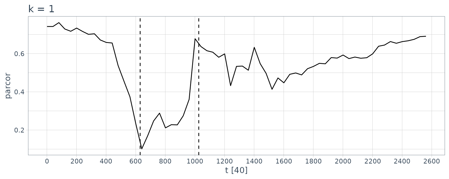
[6] "parcor"Plotting the first ar coefficient over time:
dat <- tsibble(
  parcor = fit$parcor[1, ],
  t = seq(1, nrow(MYE1F), by = 40),
  index = t
)
For \(k = 2\):
fit <- tvar(
  MYE1F,
  trend.order = 2,
  ar.order = 8,
  span = 40,
  tau2.ini = 6.6e-06,
  delta = 1.0e-06
)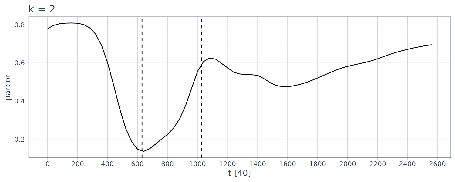
From the figure, we see that the estimated coefficients vary with time corresponding to the arrivals of the P-wave and the S-wave at n = 630 and n = 1026, respectively, which were estimated by using the locally stationary AR model.
The estimates for k = 2 are very smooth. However, as is apparent in the figure, the estimates with k = 2 cannot reveal the abrupt changes of the time series that correspond to the arrival of the P-wave and the S-wave. Compared with this, the estimates obtained from the model with k = 1 have larger fluctuations. According to the AIC, the model with k = 1 is considered to be a better model than that with k = 2. In later section, we shall consider a method of obtaining smooth estimates that also has the capability to adapt to abrupt structural changes.
Estimation of the Time-Varying Spectrum
For a stationary AR model, the power spectrum is given by:
\[\begin{aligned} p(f)&= \frac{\sigma^{2}}{\Big|1 - \sum_{j=1}^{m}a_{j}e^{-2\pi i j f}\Big|^{2}} \end{aligned}\] \[\begin{aligned} -\frac{1}{2} \leq f \leq \frac{1}{2} \end{aligned}\]Therefore, for the time-varying coefficient AR model with time-varying AR coefficients \(a_{nj}\), the instantaneous spectrum at time \(n\) can be defined by:
\[\begin{aligned} p_{n}(f) &= \frac{\sigma^{2}}{\Big|1 - \sum_{j=1}^{m}a_{nj}e^{-2\pi i j f}\Big|^{2}} \end{aligned}\]Thus, using the time-varying AR coefficients \(a_{nj}\) introduced in the previous section, we can estimate the time-varying power spectrum as a function of time, which is called the time-varying spectrum.
Example: Time-varying spectrum of a seismic data
The R function tvspc of the package TSSS computes time-varying spectrum using the outputs from the function tvar.
The inputs to the function are:
- arcoef: time-varying AR coefficients.
- sigma2: variance of the observation noise.
- span: local stationary span.
- nf: number of frequencies in computing spectrum.
For \(k = 1\):
fit <- tvar(
  dat,
  trend.order = 1,
  ar.order = 8,
  span = 20,
  tau2.ini = 1.0e-03,
  delta = 1.0e-04,
  plot=F
)

fit_var <- tvvar(
  dat,
  trend.order = 1,
  tau2.ini = 6.6e-06,
  delta = 1.0e-06
)

spec <- tvspc(
  fit$arcoef,
  fit$sigma2,
  span = 20,
  nf = 400
)

plot(
  spec,
  tvv = fit_var$tvv,
  dx = 2,
  dy = 0.10
)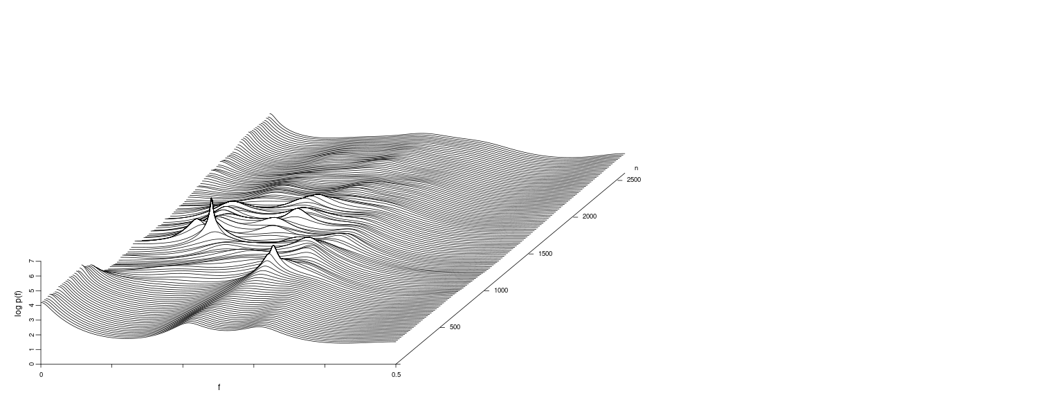
For \(k = 2\):
fit <- tvar(
  dat,
  trend.order = 2,
  ar.order = 8,
  span = 20,
  tau2.ini = 1.0e-03,
  delta = 1.0e-04,
  plot=F
)

fit_var <- tvvar(
  dat,
  trend.order = 2,
  tau2.ini = 6.6e-06,
  delta = 1.0e-06
)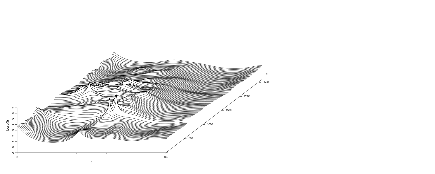
The horizontal and the vertical axes indicate the frequency and the logarithm of the spectra, respectively, and the slanted axis indicates time.
From the figures, it can be seen that the power of the spectrum around f = 0.25 increases with the arrival of the P-wave. Subsequently, the power around f = 0.1 increases with the arrival of the S-wave. After that, the peaks of the spectra gradually shift to the right, and the spectrum eventually converges to that of the original background motions.
The Assumption on System Noise for the Time-Varying Coefficient AR Model
The covariance matrix for the system noise is assumed to be a diagonal form given by:
\[\begin{aligned} \textbf{Q} &= \begin{bmatrix} \tau^{2} & &\\ & \ddots &\\ & & \tau^{2} \end{bmatrix} \end{aligned}\]At first glance, this appears to be a very strong unrealistic assumption. However, this section shows that it can be obtained naturally by considering the smoothness of the frequency response function of the AR operator.
Firstly, we consider the Fourier transform of the AR coefficients of the TVAR model:
\[\begin{aligned} A(f, n) &= 1 - \sum_{j=1}^{m}a_{nj}e^{-2\pi i j f} \end{aligned}\]This is the frequency response function of the AR model considered as a whitening filter.
Recall earlier that the frequency response function is the fourier transform of the impulse response function:
\[\begin{aligned} \sum_{j=0}^{\infty}g_{j}e^{-2\pi i j f} &= \frac{1 - \sum_{j=1}^{l}b_{j}e^{-2\pi ijf}}{1 - \sum_{j=1}^{m}a_{j}e^{-2\pi i j f}} \end{aligned}\]Then the time-varying spectrum can be expressed as:
\[\begin{aligned} p_{n}(f) &= \frac{\sigma^{2}}{|A(f, n)|^{2}} \end{aligned}\]Since the characteristics of the power spectrum are determined by the frequency response function \(A(f, n)\), we can obtain good estimates of the time-varying spectrum by controlling the smoothness of \(A(f, n)\). By considering the smoothness of \(A(f, n)\) with respect to n, we can obtain the following models for the time change of the AR coefficients.
Considering the k-th difference of the \(A(f, n)\) to evaluate the smoothness of the time change of the AR coefficients, we obtain:
\[\begin{aligned} \Delta^{k} A(f, n) &= \sum_{j=1}^{m}\Delta^{k}a_{nj}e^{-2\pi i j f} \end{aligned}\]Then taking the integral of the square, we obtain:
\[\begin{aligned} \int_{-\frac{1}{2}}^{\frac{1}{2}}|\Delta^{k}A(f, n)|^{2}\ df &= \sum_{j=1}^{m}(\Delta^{k}a_{jn})^{2} \end{aligned}\]Therefore, it is possible to curtail the change over time of the power spectrum, by reducing the sum of the squares of the k-th differences of the AR coefficients. Since the squares of the k-th differences of the AR coefficients add up with the same weights in above equation, this is equivalent to making the natural assumption that:
\[\begin{aligned} \tau_{11}^{2} &= \cdots = \tau_{mm}^{2} = \tau^{2} \end{aligned}\]And that:
\[\begin{aligned} \Delta_{n}^{k}a_{jn} &= v_{nj} \end{aligned}\] \[\begin{aligned} v_{nj} &\sim N(0, \tau^{2}) \end{aligned}\] \[\begin{aligned} j = 1, \cdots, m \end{aligned}\]Abrupt Changes of Coefficients
For the seismic data, it can be seen that the behavior of the wave form changes abruptly as a new signal arrives at a certain time. In this case, the estimated time-varying coefficients often become too variable or too smooth to capture the change of the characteristics.
In such a case, by applying the locally stationary AR model, we can obtain estimates of the change points. By using the estimates of arrival times of a new signal, it is possible to obtain better estimates of the time-varying AR coefficients.
Assume that abrupt changes are detected at times \(n = n_{1}, \cdots, n_{p}\). Corresponding to these points, the noise term \(v_{nj}\) takes a large negative or positive value. This indicates that it is necessary to increase the variance \(\tau^{2}\) at the change time points.
When \(\tau^{2}\) is increased in this way, the absolute value of the k-th time-difference of \(a_{nj}\) becomes larger. Thus, for k = 1, the coefficient \(a_{nj}\) shows a stepwise behavior and produces a discontinuous point. On the other hand, for k = 2, the slope of \(a_{nj}\) changes abruptly and yields a bending point. To yield a jump for a model with \(k \geq 2\), it is necessary to add noise to each component of the state vector. Therefore we can realize the jump either by initializing the state and the covariance matrix \(\textbf{x}_{n\mid n−1}\) and \(\textbf{V}_{n\mid n−1}\) or by adding a large positive value to all diagonal elements of \(\textbf{V}_{n\mid n−1}\) for \(n = n_{1}, \cdots, n_{p}\). This method is applicable to trend estimation as well as for the time-varying coefficient modeling.
Example: Time-varying spectrum with abrupt structural changes
To treat abrupt structural changes in the function tvspec, we specify the location of the change points by using the parameter outlier as follows:
dat <- as.ts(
  MYE1F |>
    select(value)
)

fit <- tvar(
  dat,
  trend.order = 2,
  ar.order = 8,
  span = 20,
  outlier = c(630, 1026),
  tau2.ini = 6.6e-06,
  delta = 1.0e-06,
  plot = FALSE
)

spec <- tvspc(fit$arcoef, fit$sigma2)

fit_var <- tvvar(
  dat,
  trend.order = 2,
  tau2.ini = 6.6e-06,
  delta = 1.0e-06,
  plot = FALSE
)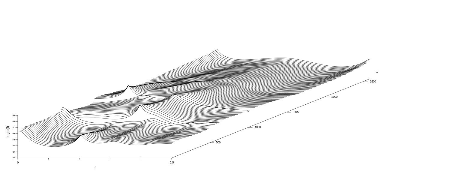
The figure above shows the time-varying AR coefficients and the time-varying spectrum estimated by the model with k = 2 and m = 4 and by assuming that sudden structural changes occur at n = 630 and n = 1026 corresponding to the arrivals times of the P-wave and the S-wave, respectively. The estimated coefficients jump twice at these two points but change very smoothly elsewhere.
We can observe two characteristics of the series, firstly, that the dominant frequencies gradually shift to the right after the S-wave arrives, and secondly, that the specrum at direct current \(p(f = 0)\) increases and the shape of the spectrum goes back to that of the original background microtremors.
Non-Gaussian State-Space Model
We extend the state-space model to cases where the system noise and/or the observation noise are non-Gaussian. This non-Gaussian model is applicable when there are sudden changes in the parameters caused by structural changes of the system or by outliers in the time series. For the general non-Gaussian models we consider here, the Kalman filtering and the smoothing algorithms sometimes cannot yield good estimates of the state. Even in such cases, however, we can derive an exact sequential formula for filtering and smoothing which can be implemented using numerical integration.
As shown in the previous chapters, various types of time series models can be expressed in terms of the linear-Gaussian state-space model:
\[\begin{aligned} \textbf{x}_{n} &= \textbf{Fx}_{n-1} + \textbf{Gv}_{n}\\ y_{n} &= \textbf{Hx}_{n} + w_{n} \end{aligned}\]\(\textbf{v}_{n}\) and \(w_{n}\) are Gaussian white noises.
The state-space model is a very useful tool for time series modeling, since it is a natural representation of a time series model and provides us with very efficient computational methods such as Kalman filtering and smoothing algorithms. Although many important time series models are expressible as linear-Gaussian state-space models, there are some other situations where extensions of the model are necessary, such as the case of a nonstationary time series with time-varying stochastic structure that sometimes contains both smooth and abrupt changes. While a linear-Gaussian state-space model can reasonably express gradual structural changes of nonstationary time series, it is necessary to build a complex model to properly address abrupt changes. Nonlinear systems and discrete processes cannot be adequately modeled by standard linear Gaussian state-space models.
Consider the following state-space model (same as above):
\[\begin{aligned} \textbf{x}_{n} &= \textbf{Fx}_{n-1} + \textbf{Gv}_{n}\\ y_{n} &= \textbf{Hx}_{n} + w_{n} \end{aligned}\]Where the system noise \(\textbf{v}_{n}\) and the observation noise \(w_{n}\) are white noises that follow the density functions q(v) and r(w), respectively. In contrast to the state-space models presented earlier, these distributions are not necessarily Gaussian.
For the linear-Gaussian state-space model, the Kalman filter provides a recursive algorithm for obtaining the conditional mean and the conditional covariance matrix of the state vector.
The information from the time series obtained until the time j is denoted as \(\textbf{Y}_{j} = \{ y_{1}, \cdots, y_{j} \}\). Similarly, the set of realizations of the state \(\textbf{x}_{n}\) up to time j is denoted as \(\textbf{X}_{j} = \{x_{1}, \cdots, x_{j}\}\). Further, the initial state vector \(\textbf{x}_{0}\) is assumed to be distributed according to the probability density function \(p(\textbf{x}_{0} \mid \textbf{Y}_{0})\).
Here the state estimation problem is to obtain the conditional distribution of the state vector \(\textbf{x}_{n}\), given the information \(\textbf{Y}_{m}\). There are three versions of the state estimation problem, depending on the relation between n and m. Specifically, for \(n > m\), \(n = m\) and \(n < m\), it is called the prediction problem, the filtering problem and the smoothing problem, respectively.
On the other hand, with the general non-Gaussian state-space model, the posterior state distribution cannot be completely determined by these quantities, and it is necessary to obtain the conditional densities for state estimation.
However, for the state-space models defined earlier, by using the relations:
\[\begin{aligned} p(\textbf{x}_{n} |\textbf{x}_{n-1}, \textbf{Y}_{n-1} ) &= p(\textbf{x}_{n} |\textbf{x}_{n-1})\\ p(\textbf{y}_{n} |\textbf{x}_{n} ,\textbf{Y}_{n-1} ) &= p(\textbf{y}_{n} |\textbf{x}_{n} ) \end{aligned}\]We can derive recursive formulas for obtaining the one-step-ahead predictive distribution \(p(\textbf{x}_{n} \mid \textbf{Y}_{n-1})\) and the filtering distribution \(p(\textbf{x}_{n} \mid \textbf{Y}_{n})\). Note that the following algorithm can be applied to general nonlinear state-space models:
One-step-ahead Prediction:
\[\begin{aligned} p(\textbf{x}_{n}|\textbf{Y}_{n-1}) &= \int_{-\infty}^{\infty}p(\textbf{x}_{n}, \textbf{x}_{n-1}|\textbf{Y}_{n-1}) \ d\textbf{x}_{n-1}\\ &= \int_{-\infty}^{\infty}p(\textbf{x}_{n}|\textbf{x}_{n-1}, \textbf{Y}_{n-1})p(\textbf{x}_{n-1}|\textbf{Y}_{n-1}) \ d\textbf{x}_{n-1}\\ &= \int_{-\infty}^{\infty}p(\textbf{x}_{n}|\textbf{x}_{n-1})p(\textbf{x}_{n-1}|\textbf{Y}_{n-1}) \ d\textbf{x}_{n-1} \end{aligned}\]Filtering:
\[\begin{aligned} p(\textbf{x}_{n}|\textbf{Y}_{n}) &= p(\textbf{x}_{n}|\textbf{y}_{n}, \textbf{Y}_{n-1})\\ &= \frac{p(\textbf{y}_{n}|\textbf{x}_{n},\textbf{Y}_{n-1})p(\textbf{x}_{n}|\textbf{Y}_{n-1})}{p(\textbf{y}_{n}|\textbf{Y}_{n-1})}\\ &= \frac{p(\textbf{y}_{n}|\textbf{x}_{n})p(\textbf{x}_{n}|\textbf{Y}_{n-1})}{p(\textbf{y}_{n}|\textbf{Y}_{n-1})} \end{aligned}\]Where the denominator can be obtained by:
\[\begin{aligned} p(\textbf{y}_{n}|\textbf{Y}_{n-1}) &= \int p(\textbf{y}_{n}|\textbf{x}_{n})p(\textbf{x}_{n}|\textbf{Y}_{n-1})\ d\textbf{x}_{n} \end{aligned}\]Next, we consider the smoothing problem. Using the equation:
\[\begin{aligned} p(\textbf{x}_{n}|\textbf{x}_{n+1}, \textbf{Y}_{N}) &= p(\textbf{x}_{n}|\textbf{x}_{n+1}, \textbf{Y}_{n}) \end{aligned}\]We obtain:
\[\begin{aligned} p(\textbf{x}_{n}, \textbf{x}_{n+1}| \textbf{Y}_{N}) &= p(\textbf{x}_{n+1}|\textbf{Y}_{N})p(\textbf{x}_{n}|\textbf{x}_{n+1}, \textbf{Y}_{N})\\ &= p(\textbf{x}_{n+1}|\textbf{Y}_{N})p(\textbf{x}_{n}|\textbf{x}_{n+1}, \textbf{Y}_{n})\\ &= p(\textbf{x}_{n+1}|\textbf{Y}_{N})\frac{p(\textbf{x}_{n}|\textbf{Y}_{n})p(\textbf{x}_{n+1}|\textbf{x}_{n}, \textbf{Y}_{n})}{p(\textbf{x}_{n+1}|\textbf{Y}_{n})}\\ &= p(\textbf{x}_{n+1}|\textbf{Y}_{N})\frac{p(\textbf{x}_{n}|\textbf{Y}_{n})p(\textbf{x}_{n+1}|\textbf{x}_{n})}{p(\textbf{x}_{n+1}|\textbf{Y}_{n})} \end{aligned}\]Smoothing Formula:
\[\begin{aligned} p(\textbf{x}_{n}|\textbf{Y}_{N}) &= \int_{-\infty}^{\infty}p(\textbf{x}_{n}, \textbf{x}_{n+1}|\textbf{Y}_{N})\ d\textbf{x}_{n+1}\\ &= p(\textbf{x}_{n}|\textbf{Y}_{n})\int_{-\infty}^{\infty}\frac{p(\textbf{x}_{n+1}|\textbf{Y}_{N})p(\textbf{x}_{n+1}|\textbf{x}_{n})}{p(\textbf{x}_{n+1}|\textbf{Y}_{N})}\ d\textbf{x}_{n+1} \end{aligned}\]Numerical Computation of the State Estimation Formula
For a linear Gaussian state-space model, all the conditional distributions \(p(\textbf{x}_{n} \mid \textbf{Y}_{n−1}), p(\textbf{x}_{n} \mid \textbf{Y}_{n}), p(\textbf{x}_{n} \mid \textbf{Y}_{N})\) become normal distributions. Therefore, in that case, only the mean vectors and the covariance matrices need to be evaluated, and the above density equations become equivalent to the ordinary Kalman filter and the smoothing algorithms. However, since the conditional distribution \(p(\textbf{x}_{n} \mid \textbf{Y}_{j})\) of the state generally becomes a non-Gaussian distribution, it cannot be specified using only the mean vector and the covariance matrix.
Various algorithms have been presented, for instance, the extended Kalman filter and the second order filter, to approximate the non-Gaussian distribution by a single Gaussian distribution with properly determined mean vector and covariance matrix. In general, however, they do not perform well.
This section deals with the method of realizing the non-Gaussian filter and the non-Gaussian smoothing algorithm by numerically approximating the non-Gaussian distributions. In this approach, a non-Gaussian state density function is approximated numerically using functions such as a step function, a piecewise linear function or a spline function. Then the above equations can be evaluated by numerical computation. Since this approach requires a huge amount of computation, it used to be considered an impractical method. Nowadays, with the development of high-speed computers, those numerical methods have become practical, at least for low-dimensional systems. In this section, we approximate the density functions by simple step functions.
To be specific, the density function \(f(t)\) to be approximated is defined on a line: \(−\infty < t < \infty\). To approximate this density function by a step function, the domain of the density function is firstly restricted to a finite interval \([t_{0}, t_{d}]\), which is then divided into d subintervals. Here \(t_{0}\) and \(t_{d}\) are assumed to be sufficiently small and large numbers, respectively.
In the actual programming, we change \(t_{0}\) and \(t_{i}\) depending on the location of the density function. However, for simplicity, ends of the sub-intervals are assumed to be fixed in the following. Further, the width of the subintervals is assumed to be identical. Then the i-th point is given by \(t_{i} = t_{0} + i\Delta t\) with \(\Delta t = \frac{t_{d} − t_{0}}{d}\).
In a step-function approximation, the function \(f(t)\) is approximated by \(f_{i}\) on the subinterval \([t_{i-1},t_{i}]\). If the function \(f(t)\) is actually a step-function, it is given by \(f_{i} = f(t_{i})\). But in general, it may be defined by:
\[\begin{aligned} f_{i} &= \Delta t\int_{t_{i-1}}^{t_{i}}f(t)\ dt \end{aligned}\]Using those values, the step-function approximation of the function \(f(t)\) is specified by:
\[\begin{aligned} \{d; t_{0}, \cdots, t_{d}; f_{1}, \cdots, f_{d}\} \end{aligned}\]In the following, the approximated function is denoted by \(\tilde{f}(t)\). For the numerical implementation of the non-Gaussian filter and the smoothing formula, it is necessary to approximate the density functions:
\[\begin{aligned} \tilde{p}(t) = &\ p(\textbf{x}_{n}|\textbf{Y}_{n-1})\\ \{d; t_{0}, \cdots,\ &t_{d}; p_{1}, \cdots, p_{d}\} \end{aligned}\] \[\begin{aligned} \tilde{f}(t) = &\ p(\textbf{x}_{n}|\textbf{Y}_{n})\\ \{d; t_{0}, \cdots,\ &t_{d}; f_{1}, \cdots, f_{d}\} \end{aligned}\] \[\begin{aligned} \tilde{s}(t) = &\ p(\textbf{x}_{n}|\textbf{Y}_{N})\\ \{d; s_{0}, \cdots,\ &s_{d}; s_{1}, \cdots, s_{d}\} \end{aligned}\] \[\begin{aligned} \tilde{q}(v) = &\ q(v)\\ \{2d+1; t_{-d}, \cdots,\ &t_{d}; q_{-d}, \cdots, q_{d}\} \end{aligned}\]On the other hand, the observation noise density \(r(v)\) can be used directly without discretizing it.
Alternative approaches for numerical integrations are Gauss-Hermite polynomial integration, a random replacement of knots spline function approximation and Monte Carlo integration.
Example: Numerical Evaluation of Simplest One-Dimensional Trend Model
\[\begin{aligned} x_{n} &= x_{n-1} + v_{n}\\ y_{n} &= x_{n} + w_{n} \end{aligned}\]One-step-ahead Prediction:
For \(i = 1, \cdots, d\), compute:
\[\begin{aligned} p_{i} &= \tilde{p}(t_{i})\\ &= \int_{t_{0}}^{t_{d}}\tilde{q}(t_{i} - s)\tilde{f}(s)\ ds\\ &= \sum_{j=1}^{d}\int_{t_{j-1}}^{t_{j}}\tilde{q}(t_{i}-s)\tilde{f}(s)\ ds\\ &= \Delta t\sum_{j=1}^{d}q_{i-j}f_{j} \end{aligned}\]Filtering:
For \(i = 1, \cdots, d\), compute:
\[\begin{aligned} f_{i} &= \tilde{f}(t_{i})\\ &= \frac{r(y_{n}-t_{i})\tilde{p}_{i}(i)}{C}\\ &= \frac{r(y_{n}-t_{i})p_{i}}{C}\\ \end{aligned}\]Where the normalizing constant C is obtained by:
\[\begin{aligned} C &= \int_{t_{0}}^{t_{d}}r(y_{n}-t)\tilde{p}(t)\ dt\\ &= \sum_{j=1}^{d}\int_{t_{j-1}}^{t_{j}}r(y_{n}-t)\tilde{p}(t)\ dt\\ &= \Delta t\sum_{j=1}^{d}r(y_{n}-t_{j})p_{j} \end{aligned}\]Smoothing:
For \(i = 1, \cdots, d\), compute:
\[\begin{aligned} s_{i} &= \tilde{s}(t_{i})\\ &= \tilde{f}(t_{i})\int_{t_{0}}^{t_{d}}\frac{\tilde{q}(t_{i}- u)\tilde{s}(u)}{\tilde{p}(u)}\ du\\ &= \tilde{f}(t_{i})\sum_{j=1}^{d}\int_{t_{j-1}}^{t_{j}}\frac{\tilde{q}(t_{i}- u)\tilde{s}(u)}{\tilde{p}(u)}\ du\\ &= \Delta t f(t_{i})\sum_{j=1}^{d}\frac{q_{i-j}s_{j}}{p_{j}} \end{aligned}\]It should be noted that, in practical computation, even after the prediction step and the smoothing, the density functions should be normalized so that the value of the integral over the whole interval becomes 1.
This can be achieved, for example, by modifying \(f_{i}\) to \(\frac{f_{i}}{I(f)}\) where:
\[\begin{aligned} I(f) &= \int_{t_{0}}^{t_{d}}f(t)\ d_{t}\\ &= \Delta t(f_{1} + \cdots + f_{d}) \end{aligned}\]Non-Gaussian Trend Model
The R function ngsmth of the package TSSS performs non-Gaussian filtering and smoothing for one-dimensional state-space model with non-Gaussian noise densities. The inputs to the function are:
- y: a univariate time series.
- noisev: type of system noise density.
- 1: Gaussian (normal) distribution,
- 2: Type VII Pearson family of distribution.
- 3: two-sided exponential distribution.
- tau2: dispersion of system noise.
- bv: shape parameter of the sytem noise.
- noisew: type of system noise density.
- 1: Gaussian (normal) distribution,
- 2: Type VII Pearson family of distribution.
- 3: two-sided exponential distribution.
- 4: double exponential distribution.
- sigma2: dispersion of the observation noise
- bw: shape parameter of the obserbaip noise.
- initd: type of initial distribition.
- 1: Gaussian (normal) distribution,
- 2: uniform distribution.
- 3: two-sided exponential distribution.
- k: number of intervals
- plot: logical. If TRUE (default), trend and smt are plotted
And the outputs from this function are:
- trend: 7 percentile points of smoothed posterior distribution of the trend.
- smt: smoothed density for n = 1, …, N.
The PfilterSample dataset is generated by the following process:
\[\begin{aligned} y_{n} &\sim N(\mu_{n}, 1) \end{aligned}\] \[\begin{aligned} \mu_{n} &= \begin{cases} 0 & 1 \leq n \leq 100\\ 1 & 101 \leq n \leq 200\\ -1 & 201 \leq n \leq 300\\ 0 & 301 \leq n \leq 400 \end{cases} \end{aligned}\]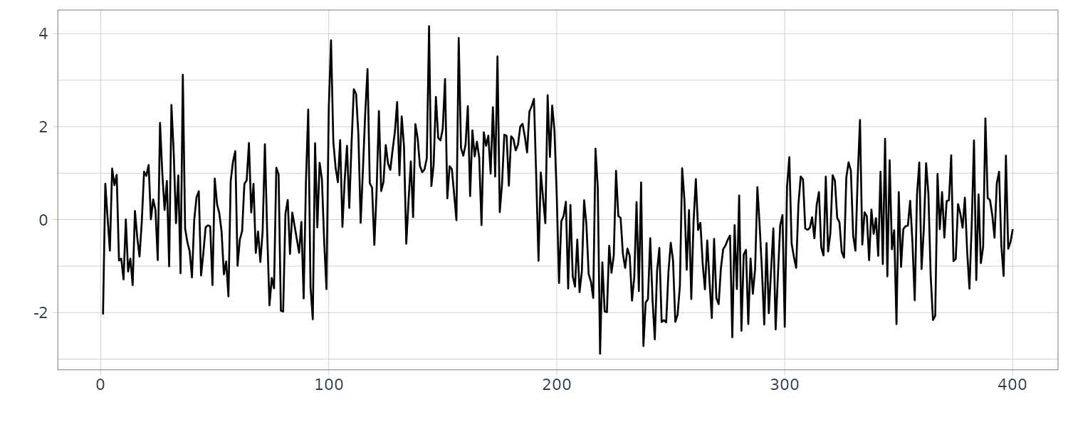
We consider the following first order trend model:
\[\begin{aligned} t_{n} &= t_{n-1} + v_{n}\\ y_{n} &= t_{n} + w_{n} \end{aligned}\]Where the observation noise \(w_{n}\) is assumed to be Gaussian, and the system noise \(v_{n}\) follows the type VII Pearson family of distributions:
\[\begin{aligned} q(v_{n}) &= \frac{c}{(\tau^{2} + v_{n}^{2})^{b}} \end{aligned}\] \[\begin{aligned} \frac{1}{2} < b < \infty \end{aligned}\]Let us try a few variety of system noise distributions:
1) Where the system noise is Gaussian (Pearson family with \(b=\infty\)):
s1 <- ngsmth(
  y,
  noisev = 1,
  tau2 = 1.4e-02,
  noisew = 1,
  sigma2 = 1.048
)

PfilterSample <- PfilterSample |>
  mutate(
    trend = s1$trend[, 4]
  )

# 3D plot
plot(
  s1,
  "smt",
  theta = 25,
  phi = 30,
  expand = 0.25,
  col = "white"
)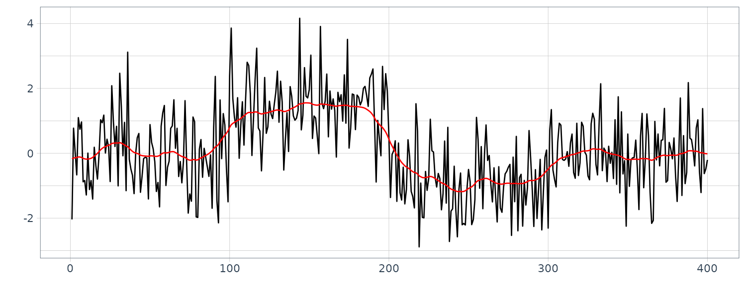
Where the system noise is Pearson family with \(b = 0.6\):
s2 <- ngsmth(
  y,
  noisev = 2,
  tau2 = 2.11e-10,
  bv = 0.6,
  noisew = 1,
  sigma2 = 1.042
)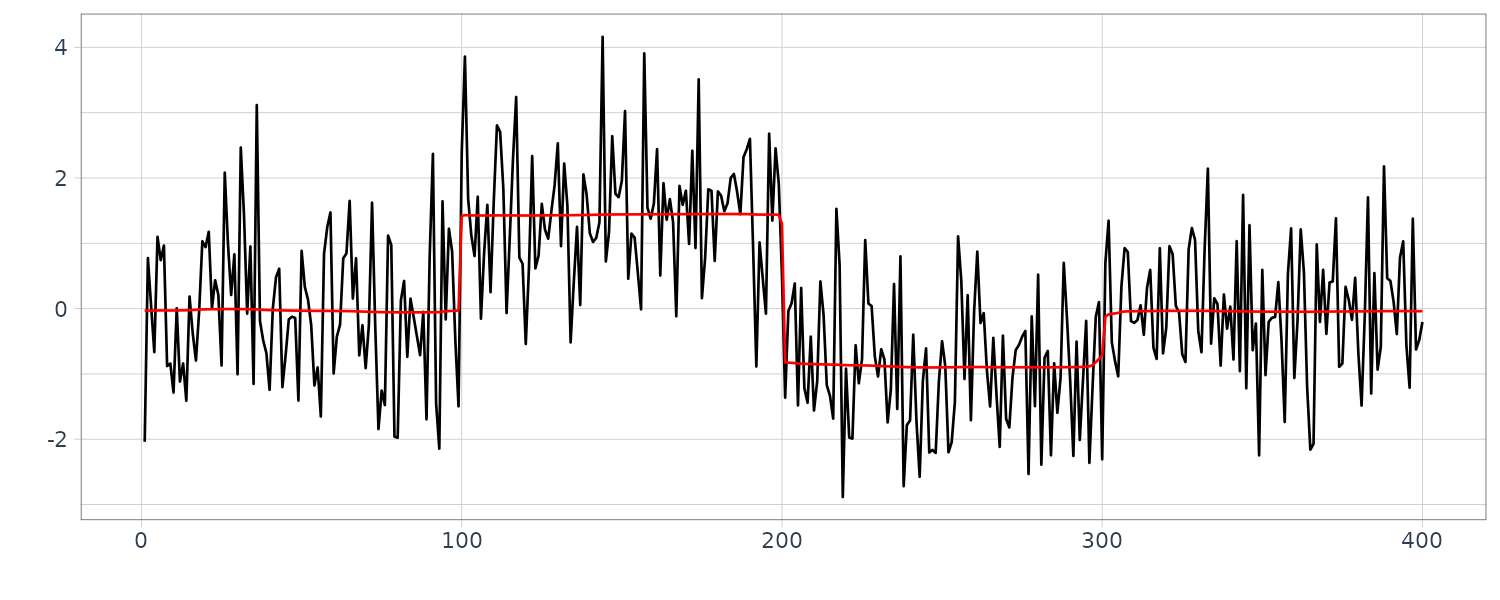

Where the system noise is Cauchy (Pearson family with \(b = 1\)):
s3 <- ngsmth(
  y,
  noisev = 2,
  tau2 = 3.53e-5,
  bv = 1.0,
  noisew = 1,
  sigma2 = 1.045
)
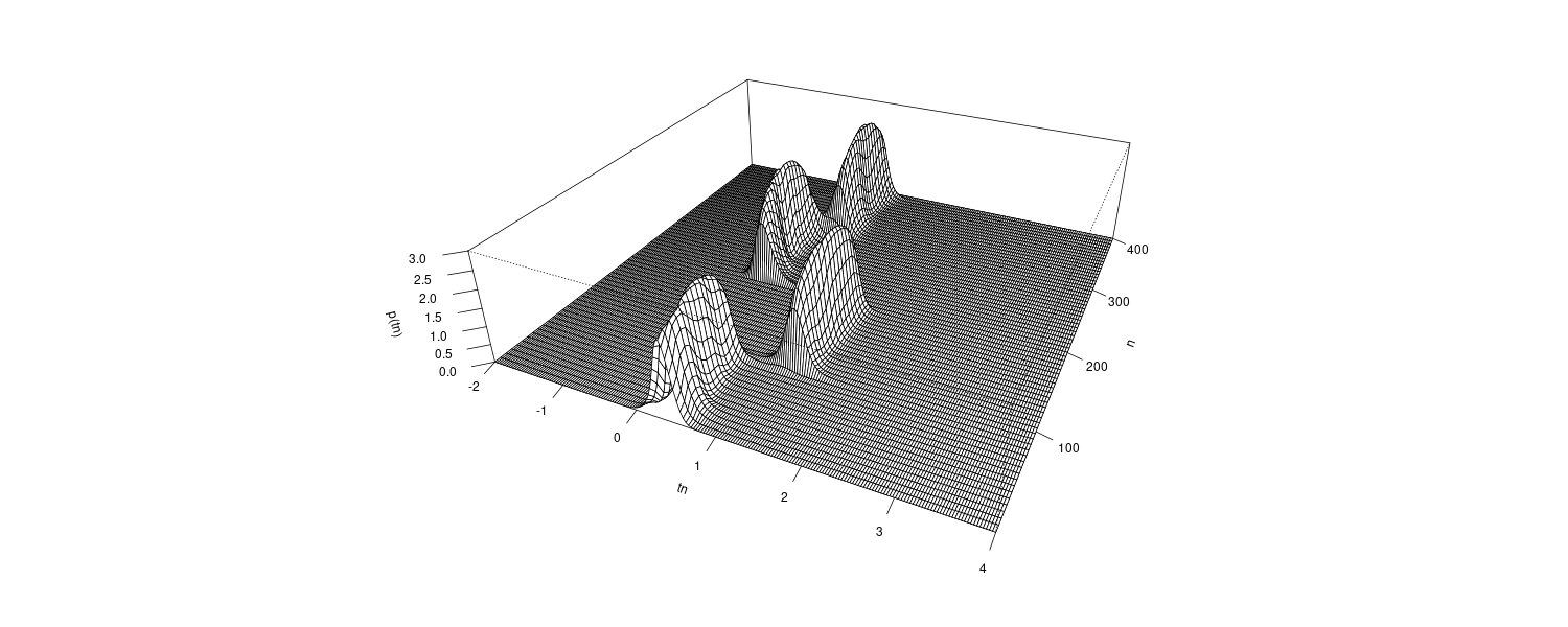
Non-symmetric Distribution – A Time-Varying Variance Model
The distribution of data observed in the real world sometimes shows non-symmetry. This is due to characteristics such as nonlinearity or non-Gaussianity of the data-generating mechanism. If we apply the least-squares method to such a dataset, we may obtain a biased estimate of the trend. Thus, if the distribution of the observations is known, we can obtain better estimates by using the non-Gaussian distribution r(w) for filtering and smoothing. In this section, for the estimation of the time-varying variance, we re-consider the model:
\[\begin{aligned} t_{m} &= t_{m-1} + v_{m} \end{aligned}\] \[\begin{aligned} y_{m} &= t_{m} + w_{m} \end{aligned}\]The R function ngsmth of the package TSSS is also applicable for the filtering and smoothing with non-Gaussian state-space model with non-symmetric noise distribution.
Example
In the previous time-varying variance example, the double exponential distribution for the observation noise \(w_{n}\) is approximated by a Gaussian distribution:
\[\begin{aligned} N\Big(\xi, \frac{\pi^{2}}{6}\Big) \end{aligned}\]Here we shall compare the smoothing results obtained by this Gaussian approximation with the one based on the exact double-exponential distribution model using non-Gaussian filter and smoother.
The plotted data set was obtained by sampling every two points after filtering by:
\[\begin{aligned} \tilde{y}_{n} &= y_{n} - 0.5 y_{n-1} \end{aligned}\]And transformed by the method discussed earlier. Since it is assumed that the time series is a white noise, this transformation was applied in order to weaken the strong autocorrelation that can be observed in the first part of the data.
n <- nrow(MYE1F)

# data transformation
yy <- rep(0, n)
for (i in 2:n) {
  yy[i] <- MYE1F$value[i] - 0.5 * MYE1F$value[i - 1]
}

m <- seq(1, n, by = 2)
y <- yy[m]
z <- tvvar(
  y,
  trend.order = 2,
  tau2.ini = 4.909e-02,
  delta = 1.0e-06
)

dat <- tsibble(
  sm = z$sm,
  t = 1:650,
  index = t
)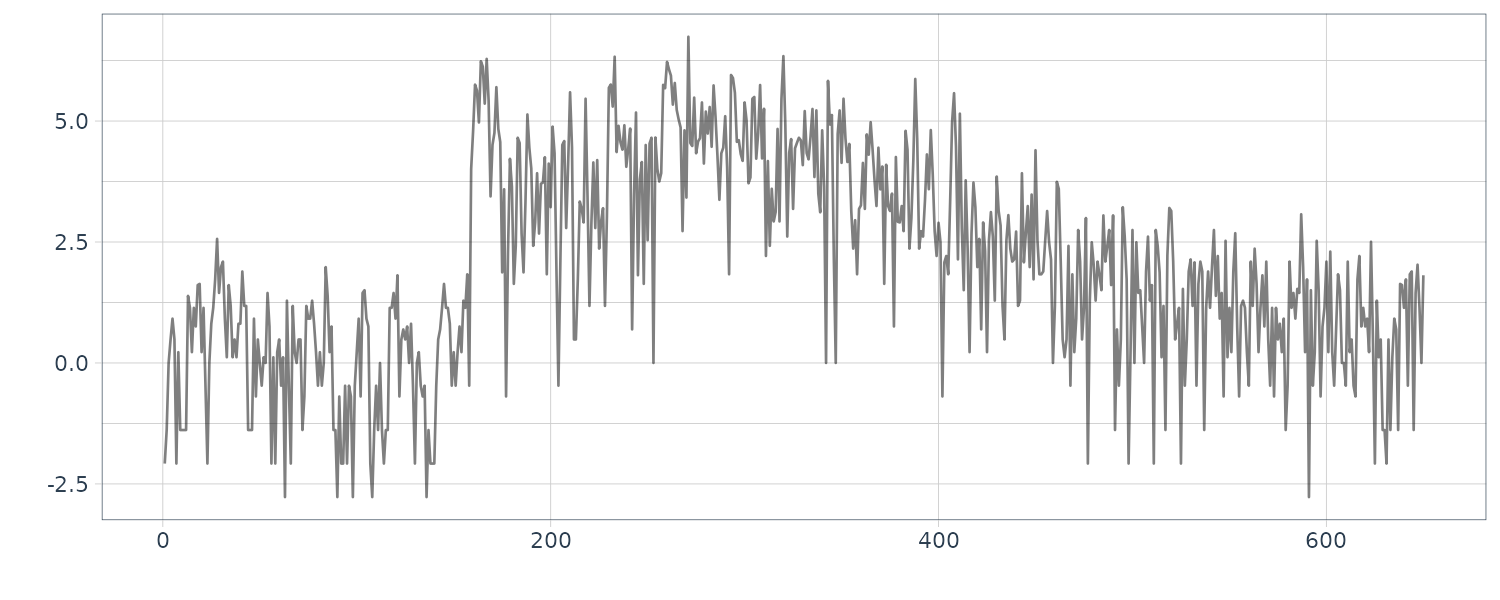
Fitting the Gaussian model with \(\sigma^{2} = \frac{\pi^{2}}{6}\) to the data:
s4 <- ngsmth(
  z$sm,
  noisev = 1,
  tau2 = z$tau2,
  noisew = 1,
  sigma2 = pi * pi / 6,
  k = 190
)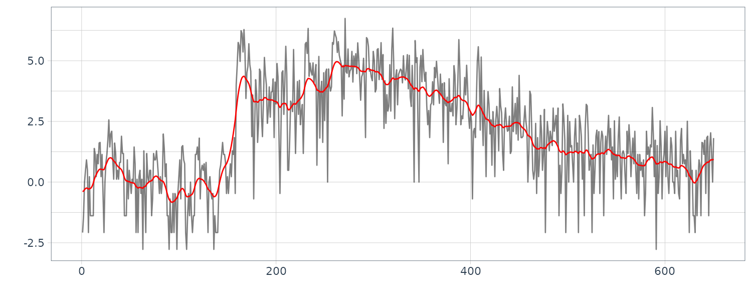

We obtain the maximum likelihood estimate \(\tau^{2} = 0.04909\) and AIC = 2165.10. The above figure shows the wiggly trend estimated by this model. This is due to the large deviations to the negative side, which occured due to the transformation, which strongly affect the estimated trend.
Fitting the non-Gaussian model with a Cauchy distribution for the system noise and a double exponential distribution for the observation noise:
\[\begin{aligned} q(x) &= \frac{1}{\pi}\frac{\tau}{\tau^{2} + x^{2}}\\ r(x) &= e^{x - e^{x}} \end{aligned}\]s5 <- ngsmth(
z$sm,
noisev = 2,
tau2 = 2.6e-4,
noisew = 4,
sigma2 = 1.0,
k = 190
)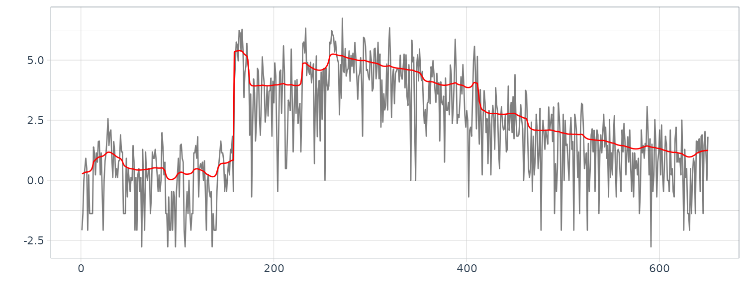

The MLE estimates are \(\hat{\tau}^{2} = 0.000260\) and AIC = 2056.97
From the big differences between the AIC values of the two models, it is evident that the non-Gaussian model is much better than the Gaussian model. The trend obtained with the non-Gaussian model is smoother by far than the one obtained by the Gaussian model and clearly detected sudden increases in the variance due to the arrivals of the P-wave and the S-wave.
In summary, by non-Gaussian smoothing with an appropriate model, we can obtain an estimate of the trend that is able to automatically detect a jump of the parameter but is not unduly influenced by a non-symmetric distribution. This estimation method of a time-varying variance can be also used for the estimation of the stochastic volatility of a financial time series as shown below.
Example: Stock Price Index Data
y <- diff(log(Nikkei225$value))

z <- tvvar(
  y,
  trend.order = 2,
  tau2.ini = 1.6e-04,
  delta = 1.0e-06
)

dat <- tsibble(
  sm = z$sm,
  t = 1:length(z$sm),
  index = t
)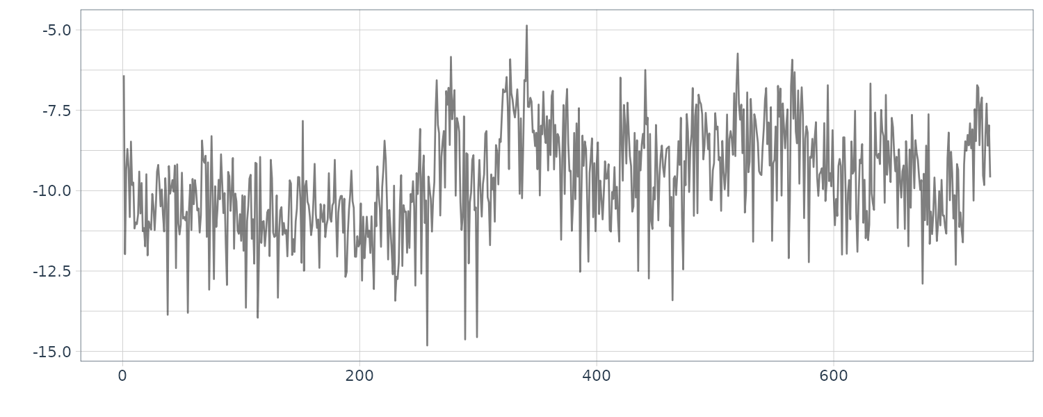
The above figure shows the transformed series sm obtained by applying the method shown earlier to the difference of the logarithm of Nikkei 225 stock price index data.
s <- ngsmth(
  z$sm,
  noisev = 1,
  tau2 = 6.9e-2,
  noisew = 4,
  sigma2 = 1.0,
  k = 190
)

s2 <- s$trend
s3 <- exp(s2[, 2] / 2) 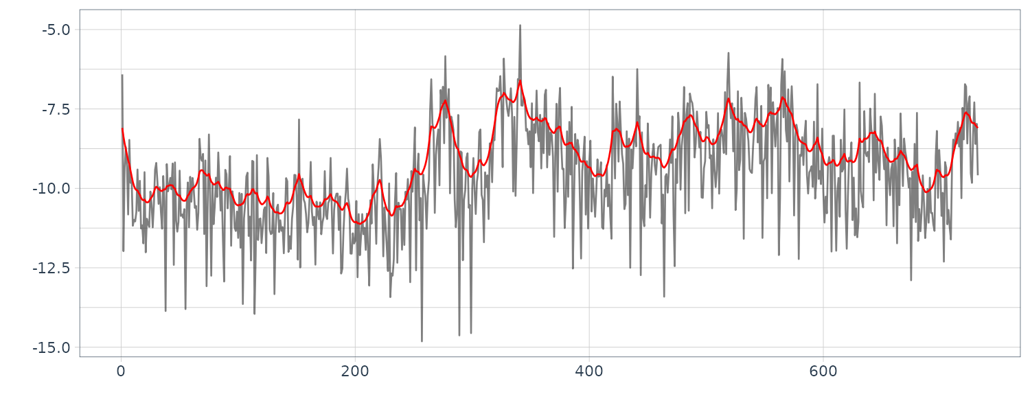
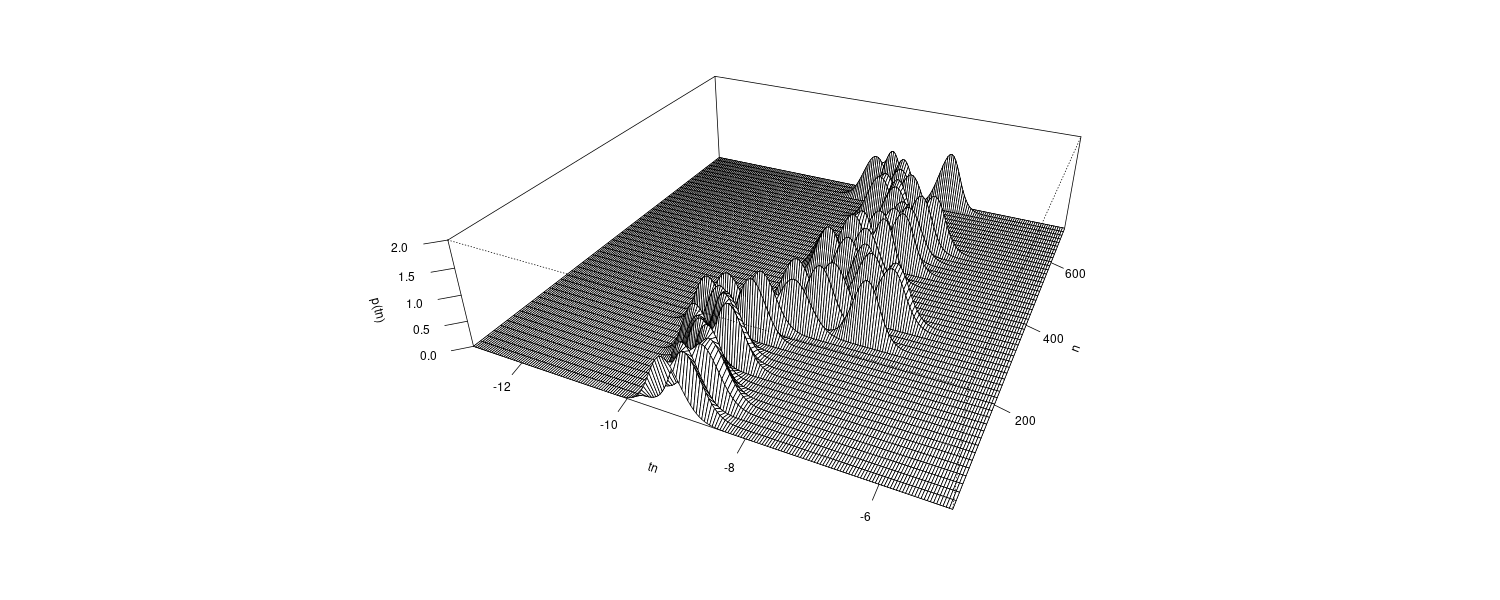
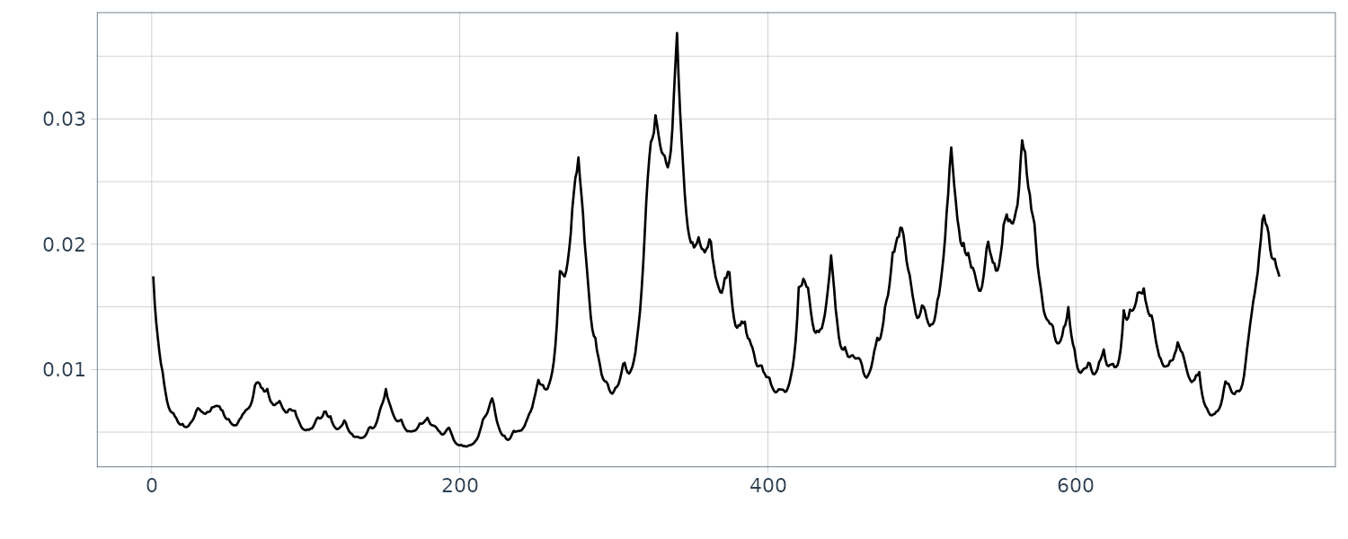
The above plot shows the posterior distribution of the estimate of \(\log \sigma_{n}^{2}\) obtained as the trend of this series estimated by the non-Gaussian model. In addition, an estimate of the volatility is obtained from the exponential of a half of the central (the 50 percentile) curve:
\[\begin{aligned} e^{\frac{\log \hat{\sigma}_{n}^{2}}{2}} &= \sqrt{\hat{\sigma}_{n}^{2}}\\ &= \hat{\sigma}_{n} \end{aligned}\]This method of estimating time-varying variance can be immediately applied to the smoothing of the periodogram. Since the periodogram follows the \(\chi^{2}\) distribution with 2 degrees of freedom, the series obtained by taking the logarithm of the periodogram thus follows the same distribution as given:
\[\begin{aligned} q(x) &= \frac{1}{\pi}\frac{\tau}{\tau^{2} + x^{2}}\\ r(x) &= e^{x - e^{x}} \end{aligned}\]Therefore, the method treated in this section can be applied to smoothing of the logarithm of the periodogram as well.
Moreover, using a non-Gaussian model, it is possible to estimate the time-varying variance from the transformed data
\[\begin{aligned} z_{n} &= \log y_{n}^{2} \end{aligned}\]In this case, for the density function of the observation noise, we use the density function obtained as the logarithm of the \(\chi^{2}\) distribution with 1 degree of freedom:
\[\begin{aligned} r(w) &= \frac{1}{\sqrt{2\pi}}e^{\frac{w - e^{w}}{2}} \end{aligned}\]Here the time-varying variance can be estimated without making the assumption that \(\log \sigma_{2m-1}^{2} = \log \sigma_{2m}^{2}\).
Applications of the Non-Gaussian State-Space Model
In this section, several applications of the non-Gaussian state-space model are presented. Specifically, modeling for processing outliers, smoothing for discrete processes and a direct method for estimating time-varying variances are shown. Extension to nonlinear state-space modeling is also shown.
Processing of the outliers by a mixture of Gaussian distributions
Here we consider treatment of outliers that follow a distribution different from the usual noise distribution of observations. To treat outliers in a time series, assuming that the outliers appear with low probability \(\alpha << 1\), it will be reasonable to use a Gaussian mixture distribution for the observation noise \(w_{n}\):
\[\begin{aligned} r(w) &= (1 - \alpha)\psi(w; \mu, \sigma^{2}) + \alpha \psi(w;\xi, \delta^{2}) \end{aligned}\]Here \(\psi(x; \mu, \sigma^{2})\) denotes the density function of the normal distribution with mean \(\mu\) and variance \(\sigma^{2}\). The first and second terms on the right-hand side express the distributions of the normal observations and the outliers, respectively.
In particular, by putting \(\xi = \mu = 0\) and \(\delta^{2} >> \sigma^{2}\), the observation noise of the outliers is assumed to have zero mean and a large variance.
The Cauchy distribution may be considered as an approximation of the above-mentioned mixture distribution. Therefore, the outliers can be treated, for example, using the Cauchy distribution or the Pearson family of distributions, which can be used to generate a density function of the observation noise. On the other hand, if outliers always appear on the positive side of the time series, we can estimate the trend properly, ignoring the outliers by setting:
\[\begin{aligned} \xi &>> \mu \end{aligned}\] \[\begin{aligned} \delta^{2} &= \sigma^{2} \end{aligned}\]A nonstationary discrete process
Non-Gaussian models can also be applied to the smoothing of discrete processes, for instance, nonstationary binomial distributions and Poisson distributions.
Consider the time series \(m_{1}, \cdots, m_{N}\) that takes integer values. Assume that the probability of taking value \(m_{n}\) at time n is given by the Poisson distribution:
\[\begin{aligned} P(m_{n}|p_{n}) &= \frac{e^{-p_{n}}p_{n}^{m_{n}}}{m_{n}!} \end{aligned}\]Where \(p_{n}\) denotes the expected frequency of the occurrences of a certain event at a unit time. In this model, it is implicitly assumed that the mean of the Poisson distribution is not a constant but gradually changes with time. Such a model is called a nonstationary Poisson process model. As a model for the change over time of the Poisson mean, \(p_{n}\), we may use the trend component model:
\[\begin{aligned} p_{n} &= p_{n-1} + v_{n} \end{aligned}\]Here, since \(p_{n}\) is required to be positive, \(0 < p_{n} < \infty\), we define a new variable:
\[\begin{aligned} \theta_{n} &= \log p_{n} \end{aligned}\]And apply a trend component model for \(\theta_{n}\). Therefore, the model for smoothing the nonstationary Poisson process becomes:
\[\begin{aligned} \theta_{n} &= \theta_{n-1} + v_{n} \end{aligned}\] \[\begin{aligned} P(m_{n}|\theta_{n}) &= \frac{e^{-p_{n}}p_{n}^{m_{n}}}{m_{n}!} \end{aligned}\]Where \(p_{n}\) is defined by:
\[\begin{aligned} p_{n} &= e^{\theta_{n}} \end{aligned}\]The first and second models correspond to the system model and the observation model, and yield conditional distributions of \(\theta_{n}\) and \(m_{n}\), respectively. Therefore the non-Gaussian filtering method can be applied to the discrete process, and we can estimate the time-varying Poisson mean value from the data.
Similarly, the non-Gaussian state-space model can be applied to the smoothing of an inhomogeneous binary process. Assume that the probability of a certain event occurring \(m_{n}\) times in the \(l_{n}\) observations at time n is given by the binomial distribution:
\[\begin{aligned} P(m_{n}|p_{n}, l_{n}) &= {l_{n}\choose m_{n}}p_{n}^{m_{n}}(1 - p_{n})^{l_{n}- m_{n}} \end{aligned}\]Here, \(p_{n}\) is called the binomial probability, and expresses the expected number of occurrences of a certain event. In this case, if \(p_{n}\) varies with time, this model is called the inhomogeneous binary process model. \(p_{n}\) can be estimated by the following model:
\[\begin{aligned} \theta_{n} &= \theta_{n-1} + v_{n}\\ P(m_{n}|\theta_{n}, l_{n}) &= {l_{n}\choose m_{n}}p_{n}^{m_{n}}(1 - p)^{l_{n}-m_{n}} \end{aligned}\] \[\begin{aligned} p_{n}&= \frac{e^{\theta_{n}}}{1 + e^{\theta_{n}}} \end{aligned}\]A direct method of estimating the time-varying variance
Previously, the time-varying variance was estimated by smoothing the logarithm of the square of the original time series. However, it is also possible to estimate the time-varying variance directly using the following model:
\[\begin{aligned} t_{n} &= t_{n-1} + v_{n} \end{aligned}\] \[\begin{aligned} y_{n} &\sim N(0, e^{t_{n}}) \end{aligned}\]Since the variance always takes a positive value in this model, the state \(t_{n}\) can be taken as the logarithm of the variance. Here, \(e^{t_{n}}\) becomes an estimate of the variance at time n. From the estimation of the time-varying variance of the Nikkei 225 stock price index data, we can obtain equivalent results. Here the obtained log-likelihood values for each model are different. This is because the data sets used in computing the log-likelihood are different. We can confirm that these two models have exactly the same AIC values by compensating for the effect of data transformation by evaluating the Jacobian of the transformation.
Nonlinear State-Space Models
Consider a system described by a nonlinear state-space model:
\[\begin{aligned} \textbf{x}_{n} &= f(\textbf{x}_{n-1}) + \textbf{w}_{n}\\ y_{n} &= h(\textbf{x}_{n}) + e_{n} \end{aligned}\]Where \(y_{n}\) and \(\textbf{x}_{n}\) are one-dimensional time series and m-dimensional state vectors, respectively, and \(f(\textbf{x})\) and \(h(\textbf{x})\) are nonlinear functions of the state \(\textbf{x}\). \(\textbf{w}_{n}\) and \(e_{n}\) are m-dimensional and one-dimensional white noise sequences having densities \(q(\textbf{w})\) and \(r(e)\), respectively, which are independent of the past history of \(\textbf{x}_{n}\) and \(y_{n}\). The initial state vector \(\textbf{x}_{0}\) is assumed to be distributed according to the density \(p(\textbf{x}_{0})\).
For the nonlinear state-space model, the conditional distributions are given by:
\[\begin{aligned} p(\textbf{x}_{n}|\textbf{x}_{n-1}) &= q(\textbf{x}_{n} - f(\textbf{x}_{n-1}))\\ p(y_{n}|\textbf{x}_{n}) &= r(y_{n} - h(\textbf{x}_{n})) \end{aligned}\]Further, it can be verified that the following relations hold:
\[\begin{aligned} p(\textbf{x}_{n}|\textbf{x}_{n-1}, \textbf{Y}_{n-1}) &= p(\textbf{x}_{n}|\textbf{x}_{n-1})\\ p(y_{n}|\textbf{x}_{n}, \textbf{Y}_{n-1}) &= p(y_{n}|\textbf{x}_{n})\\ p(\textbf{x}_{n}|\textbf{x}_{n+1}, \textbf{Y}_{N}) &= p(\textbf{x}_{n}|\textbf{x}_{n+1}, \textbf{Y}_{n}) \end{aligned}\]The non-Gaussian filtering and smoothing methods can be also applied for nonlinear state-space model.
