In this post, we will cover Matsuura K. (2023) Bayesian Statistical Modeling with Stan, R, and Python.

The returned result, d_ms is a data frame with the size of (number of draws) × (number of the variables). By default, draws from the warmup period are not included. As an example, let us check the draws of the slope b and compute its 95% Bayesian confidence interval. We can use quantile function to compute the 95% interval because d_ms$b is a numeric vector:

> quantile(d_ms$b, probs=c(0.025, 0.975))
2.5% 97.5%
0.5540 0.9525

Bayesian Confidence Intervals and Bayesian Prediction Intervals

Let us first generate the draws from these distributions:

N_ms <- nrow(d_ms)
y10_base <- d_ms$a + d_ms$b * 10
y10_pred <- rnorm(
  n = N_ms,
  mean = y10_base,
  sd = d_ms$sigma
)

ideally, we want to compute the various quantities in Stan. transformed parameters block and generated quantities block can be used for this purpose

data {
  int N;
  vector[N] X;
  vector[N] Y;
  int Np;
  vector[Np] Xp;
}

parameters {
  real a;
  real b;
  real<lower=0> sigma;
}

transformed parameters {
  vector[N] y_base = a + b*X[1:N];
}

model {
  Y[1:N] ~ normal(y_base[1:N], sigma);
}

generated quantities {
  vector[Np] yp_base = a + b*Xp[1:Np];
  array[Np] real yp = normal_rng(yp_base[1:Np], sigma);     
}

Note that the normal_rng function cannot return a vector but reals, which means an array of real, the declaration must be array[Np] real. The main differences between array and vector are that array can store integers, but vectorized operations, notations, and functions for vectors cannot be used.

Terminologies Used in the Book

Probability Distribution

Probability distribution is the expression of how likely a random variable takes each of the possible values. It also can be simply called as distributions. The probability distribution of random variable a is written as p(a).

When the random variable is a discrete variable, the probability distribution is called a probability mass function (pmf).

When the random variable is a continuous variable, the probability distribution is called a probability density function. It is also called a density. Note that if the probability density function is denoted as p(x), the value at p(x) (for instance, p(x = 0)) is not a probability. Rather, the integral of p(x) is a probability. For instance, the probability that $0 \leq x \leq 0.2$ can be expressed as follows:

\[\begin{aligned} \int_{0}^{0.2}p(x)\ dx \end{aligned}\]

Joint Distribution

When there are multiple random variables, a joint distribution expresses the probability that how likely each of these random variables takes the possible values for them. It is a type of probability distribution. When there are two random variables a and b, we write their joint distribution as p(a, b), and when we have total of K random variables:

\[\begin{aligned} \theta_{1}, \theta_{2}, \cdots, \theta_{K} \end{aligned}\]

We write their joint distribution as:

\[\begin{aligned} p(\theta_{1}, \theta_{2}, \cdots, \theta_{K}) \end{aligned}\]

Marginal Distribution

Marginalization is the elimination of variables by summing up or integrating a joint distribution with respect to random variables in the joint distribution over their possible values. The probability distribution obtained by marginalization is called a marginal distribution. For instance, by summing up the joint probability with respect to a discrete random variable a, we can obtain the marginal distribution p(b) from p(a, b):

\[\begin{aligned} p(b) &= \sum_{a}p(a, b) \end{aligned}\]

Similarly, when a is a continuous random variable, by integrating the joint distribution with respect to a, we can obtain the marginal distribution p(b) from p(a, b):

\[\begin{aligned} p(b) &= \int p(a, b)\ da \end{aligned}\]

Conditional Probability Distribution

We consider a joint distribution p(a, b). The distribution of the random variable a, when a value $b_{0}$ is given to the random variable b, is called the conditional probability distribution, and is written as $p(a\mid b_{0})$. The following equation holds true:

\[\begin{aligned} p(a\mid b_{0}) &= \frac{p(a, b_{0})}{p(b_{0})} \end{aligned}\]

In addition, when the location and the shape of the probability distribution of a random variable y is determined by parameter $\theta$, we write it as $p(y\mid \theta )$.

Independence

When we say that two random variables a and b are mutually independent, we mean that this equation holds true:

\[\begin{aligned} p(a, b) = p(a)p(b) \end{aligned}\]

Further, from the definition of conditional probability distribution, this is equivalent to:

\[\begin{aligned} p(a|b) = p(a) \end{aligned}\]

Partial Derivative

Consider a function of two variables $f(\theta_{1}, \theta_{2})$. We consider the derivative by fixing $\theta_{2}$ as a constant and changing $\theta_{1}$:

\[\begin{aligned} \lim_{\Delta theta_{1} \rightarrow 0}\frac{f(\theta_{1} + \Delta\theta_{1}, \theta_{2}) - f(\theta_{1}, \theta_{2})}{\Delta \theta_{1}} \end{aligned}\]

And this is called partial derivative of $f(\theta_{1}, \theta_{2})$ with respect to $\theta_{1}$. The same would apply for multivariate function $f(\theta_{1}, \theta_{2}, \cdots, \theta_{K})$, and when taking its derivative, we only need to consider all variables as constants, except for $\theta_{1}$.

Overview of Statistical Modeling

Statistical modeling is an analysis method that promotes understanding and prediction of phenomena by fitting probabilistic models to the data of interest. A probabilistic model consists of probability distributions, parameters, and mathematical expressions representing relations between the parameters. A parameter is a variable whose value is unknown before conducting analysis. The values of parameters in a probabilistic model are estimated from data, and these values are further used to interpret and predict the phenomenon of interest.

The first purpose of statistical modeling is interpretation. It is one of the fundamental human nature that we want to know the reasonings and mechanisms of phenomena, and to acquire new knowledge. Modeling plays a role in facilitating the understanding of how the phenomenon occurred and how the data was generated. From this point of view, models that are easy to interpret are considered as good models. Such models can also be said to be convincing, oreasy-to-explain models. Ease of interpretation makes the decision making easier.

The second purpose of statistical modeling is prediction. That is, to predict the future output of the phenomenon using the obtained data, or to predict how the system responds to a new input. From this point of view, models with high accuracy of prediction are regarded as good models.

Note that interpretation and prediction are not independent of each other. A convincing model that is consistent with domain knowledge is generally robust. The term robustness is used to represent a model property that interpretation and prediction will not change largely when there are slight changes to the model or to the input data. Thus, a model with low robustness often fails to predict against new data sets. This leads to a substantial failure in practice.

Recommended Statistical Modeling Workflow

The key to follow this workflow is to start from a simple model. When we try to handle real-world data, we tend to assume a complex mechanism from the very first. However, we may end up being stuck there and not able to move on to the next step. Or even if we succeed implementing the model, parameter estimation may not work. To avoid such issues, it is a common practice to try from a simple model. Here are some suggestions as examples:

If it is possible to use a simple model that is frequently used in textbooks in the field, start from that simple model.
If there are many explanatory variables, narrow them down.
Treat random variables as independent as possible. For instance, use univariate distributions instead of multivariate distributions.
Ignore group differences or individual differences in the first model.

After starting from a simple model that works fine, repeat all or parts of the above workflow several times in cycles, gradually make it a more complex model. It seems to be a circuitous at first glance, but it enables us to find any improper assumptions. Also, by doing this, there will be less possibility introducing bugs for the model. These will help to take the minimum amount of time to a successful model.

Maximum Likelihood Estimation

Let $p(y\mid \theta)$ be a probability distribution whose shape is determined by the parameter value $\theta$. Then the likelihood $L(\theta)$ is defined to be:

\[\begin{aligned} p(y = Y |\theta) \end{aligned}\]

Which is obtained by substituting data Y into the probability distribution. In the case of the above example, if we let $y_{n}$ be the random variable that corresponds to the data point Y[n], then $p(y\mid \theta)$ is the joint distribution $p(y_{1}, y_{2}, \cdots, y_{n} \mid \mu)$. Here, since $y_{1}, y_{2}, \cdots, y_{n}$ are mutually independent, the joint distribution is equivalent to:

\[\begin{aligned} p(y_{1}, y_{2}, \cdots, y_{n} \mid \mu) &= p(y_{1}|\mu)\times \cdots \times p(y_{n}\mid \mu)\\ &= N(y_{1}|\mu, 1) \times \cdots \times N(y_{n}\mid \mu, 1) \end{aligned}\]

Note that a likelihood $p(Y\mid \theta) = L(\theta)$ is a function of parameter $\theta$. A likelihood is an indicator of the goodness of fit of a model, but it is not a probability function because the integral with respect to θ is not necessarily 1.

In general, a likelihood has a very small value because it is the product of many values that are smaller than 1. As a result, computing such small number in a computer can be problematic. Therefore, it is common to take logarithm of a likelihood for estimation, i.e., a log-likelihood. For example, the log-likelihood obtained by taking the logarithm is as follows:

\[\begin{aligned} \log L(\mu) &= \sum_{n=1}^{n}\log N(y = Y_{n}|\mu, 1) \end{aligned}\]

If we only have a single parameter as in the previous example, all we have to do is to differentiate the log-likelihood with respect to $\theta$ and obtain the value of $\theta$ that maximizes that log-likelihood by solving the following equation:

\[\begin{aligned} \frac{\partial}{\partial \theta}\log L(\theta) &= 0 \end{aligned}\]

However, when the number of parameters increases, it is difficult to solve the above equation analytically. In such cases, it is necessary to use numerical calculation methods to get the maximum likelihood estimate from a computer. In a typical algorithm, the maximum likelihood estimate is calculated in two steps. First, set initial values of the parameters in a certain way. Next, move the parameters in the direction in which the log-likelihood increases most from the current position. We repeat this second step until the log-likelihood does not increase any more. As an example, optim function in R and an optimizer in TensorFlow does MLE by roughly adopting this method.

Bayesian Inference and MCMC

The difference between traditional statistics and Bayesian statistics is that Bayesian statistics assume that all parameters are random variables and follow certain probability distributions. Therefore, in the Bayesian framework, it is possible to make a clear statement such as “the probability that the value of parameter θ is in the interval [a, b] is 95%”. Also, it allows us to answer some questions such as “What is the probability that more than ten people will visit the shop tomorrow?””.

Recall that the goal of MLE is to find a particular value for the parameter $\theta$. By contrast, in Bayesian inference, we are interested in the distribution of the parameter $p(\theta \mid Y)$ after the data Y was observed. $p(\theta\mid Y)$ is called a posterior distribution, emphasizing that it is a distribution computed after the data is observed. In some contexts, it is also called a posterior probability.

Correspondingly, a distribution $p(\theta)$ before any data is observed is called a prior distribution, or a prior probability. If there are more than one parameters, the posterior distribution for these parameters $\theta_{1}, \cdots, \theta_{K}$ becomes a joint distribution $p(\theta_{1}, \cdots, \theta_{K}\mid Y)$.

In this case, $p(\theta_{1}\mid Y)$ is the posterior distribution of a single paramter $\theta_{1}$, which is obtained by marginalizing the joint distribution.

Using Bayes’ theorem, a posterior distribution can be obtained as follows:

\[\begin{aligned} p(\theta | Y) &= \frac{p(Y|\theta)p(\theta)}{P(Y)}\\ &\propto p(Y|\theta)p(\theta) \end{aligned}\]

That is, the posterior distribution $p(\theta\mid Y)$ is proportional to the product of likelihood $p(Y\mid \theta)$ and the prior distribution $p(\theta)$ . $p(Y)$ is a constant value that depends only on the observed data Y and does not depend on $\theta$. Computing the likelihood and the prior distribution is straightforward, but computing p(Y) is usually not easy. Therefore, analytical solutions for a posterior distribution are usually too complex or intractable.

MCMC enables us to obtain the posterior distributions, by performing numerical approximation. MCMC ignores the normalization constant p(Y) and draws many random values in proportion to $p(Y\mid \theta)p(\theta)$, and uses the set of these draws instead of the posterior distribution itself. In this book, the set of random draws obtained by MCMC are called aN

MCMC sample.

The MLE method search for the parameters with the largest likelihood based on the log-likelihood, whereas Bayesian inference explores the parameter space based on the log posterior probabilities obtained by log transformation of posterior probabilities. The log posterior probability is expressed by the following equation:

\[\begin{aligned} \log p(\theta|Y) &= \log p(Y|\theta) + \log p(\theta) + \text{const} \end{aligned}\]

In Stan, $\log p(Y \mid \theta) + \log p(\theta)$ is denoted as the log posterior probability (lp__), which drops the irrelevant constant term for sampling. Note that $\log p(Y \mid \theta)$ is the log-likelihood.

Two most widely known methods for drawing an MCMC sample are Metropolis–Hastings sampling and Gibbs sampling. Stan uses another method called NUTS.

All these methods start from setting initial values of the parameters. Then, they iterate the step where they update the values of all the parameters by drawing random values based on the current values. These parameter values compose an MCMC sample. A sequence of the drawn values along the number of iterations is called a chain.

In the case where the posterior distribution has poor convergence, the autocorrelation of a sequence is typically large. In other words, the value at each iteration highly depends on the value at the earlier iterations. And hence, the effective MCMC sample size does not increase. If autocorrelation is not very high, we can improve the convergence by keeping only one draw from every several iterations, a process called thinning.

Convergence assessment is critical in the Bayesian modeling process. If the posterior distribution has poor convergence, changing the initial values or the random seed would produce considerably different posterior distributions, which will cause non-reproducible results of the analysis. Therefore, if MCMC convergence is poor, the MCMC sample obtained should not be used for the further analysis.

In order to determine the efficacy of a new drug, we conducted a clinical trial with 20 patients. Assume that the result shows that the new drug successfully cured 14 patients out of 20 (i.e., Y = 14, N = 20). Suppose that the number of cured people y follows the following Binomial distribution:

\[\begin{aligned} \text{Binomial}(y |N, \theta) &= \frac{N!}{y!(N-y)!}\theta^{y}(1 - \theta)^{N- y} \end{aligned}\]

Now we are planning to conduct the second trial using the same drug for 100 patients. Based on the result from the first trial, how many patients will be cured in the second experiment? Or more generally, what is the probability that y patients will be cured by the second trial? To answer this question, we need to consider a predictive distribution of the new data, instead of the distribution of the parameters.

In the case of MLE, a predictive distribution is obtained by substituting the maximum likelihood estimate of the parameter $\theta$ into $p(y\mid \theta)$, which is the probability distribution for generating data. Mathematically, this is:

\[\begin{aligned} p_{pred}(y|Y) = p(y|\hat{\theta}) \end{aligned}\]

Such a predictive distribution is sometimes called plug-in predictive distribution. In this example, since $\theta$ is calculated as:

\[\begin{aligned} \theta &= \frac{14}{20}\\ &= 0.7 \end{aligned}\]

The predictive distribution is:

\[\begin{aligned} \text{Binomial}(y |N = 100, \theta = 0.7) &= \frac{100!}{y!(100-y)!}0.7^{y}(1 - 0.7)^{100- y} \end{aligned}\]

The limitation of this approach is that it does not take into account the uncertainty of the parameter estimation. For example, if there are 140 cured patients out of 200 in the first experiment, it still gives the same predictive distribution as the above case.

In the case of MLE, the uncertainty from the result of the first clinical trial is not being considered, and therefore, the results overfit to this particular data generated from one single trial. To avoid overfitting, a method called scenario analysis is often used. In the scenario analysis, several analyses are performed under different scenario assumptions, and in some cases, the results from different scenarios are integrated to obtain the final result.

For instance, in the above example, one would perform scenario analysis by assuming that the weight of $\theta = 0.7$ is 0.5 (scenario of MLE), the weight of $\theta = 0.5$ is 0.4 (pessimistic scenario of small clinical effect), and the weight of $\theta = 0.6$ is 0.1 (optimistic scenario of large clinical effect). The predictive distribution in this example is considered as a mixture distribution of plug-in distributions in each scenario, as follows:

\[\begin{aligned} p_{pred}(y|Y) = &\ \text{Binomial}(y |N, \theta = 0.7) \times 0.5 +\\ &\ \text{Binomial}(y |N, \theta = 0.5) \times 0.4 +\\ &\ \text{Binomial}(y |N, \theta = 0.4) \times 0.5 \end{aligned}\]

Expanding this scenario analysis, first we calculate the probabilities of all possible scenarios given the data, $p(\theta\mid Y)$, which is the posterior distribution of $\theta$. Then we use $p(\theta\mid Y)$ as the weight for each scenario, and get the weighted sum of the probability distribution for generating data $p(y\mid \theta)$. The resulting mixture distribution is a Bayesian predictive distribution. Writing it in a mathematical formula, we have:

\[\begin{aligned} p_{pred}(y|Y) &= \int p(y|theta)p(\theta|Y)\ d\theta \end{aligned}\]

In other words, the predictive distribution in Bayesian inference is the average of the probability distributions for generating data over the posterior distribution of parameters. Thus, it can be said that the predictive distribution in Bayesian inference considers the uncertainty of parameter estimates.

Using the Dirac Delta Function

Mathematically, a distribution approximated by random draws can be expressed as a mixture of the Dirac delta functions. For example, a posterior distribution can be expressed by using Dirac delta functions as follows:

\[\begin{aligned} p(\theta|Y) &= \frac{1}{N_{ms}}\sum_{i=1}^{N_{ms}}\delta(\theta - \theta_{(i)}) \end{aligned}\]

Where $N_{ms}$ is the MCMC sample size (the number of draws), and $\theta_{(i)}$ is the i-th random draw. The Dirac delta function $\delta(x)$ is a normal distribution function whose peak is extremely sharp at x = 0. It has the following property:

\[\begin{aligned} \int_{-\infty}^{\infty}f(x)\delta(x-a)\ dx &= f(a) \end{aligned}\]

By using this property, the average of $f(\theta)$ over the posterior distribution can be written as:

\[\begin{aligned} \int f(\theta)p(\theta|Y)\ d\theta &= \int f(\theta)\frac{1}{N_{ms}}\sum_{i=1}^{N_{ms}}\sum_{i=1}^{N_{ms}}\delta(\theta - \theta_{(i)})\ d\theta\\ &= \frac{1}{N_{ms}}\sum_{i=1}^{N_{ms}}f(\theta_{(i)}) \end{aligned}\]

Now let us look at the case where we express the predictive distribution as random draws. By using the property of the Dirac delta function, the predictive distribution can also be obtained by replacing the integral with the sum over draws:

\[\begin{aligned} p_pred(y|Y) &= \int p(y|\theta)p(\theta|Y)\ d\theta\\ &= \int p(y|\theta)\frac{1}{N_{ms}}\sum_{i=1}^{N_{ms}}\delta(\theta - \theta_{(i)})\ d\theta\\ &= \frac{1}{N_{ms}}\sum_{i=1}^{N_{ms}}p(y|\theta_{(i)}) \end{aligned}\]

For instance, in the above example of the clinical trials, the distribution for generating data was a Binomial distribution. Therefore, the predictive distribution becomes a mixture of Binomial distributions as follows:

\[\begin{aligned} p_{pred}(y|Y) &= \frac{1}{N_{ms}}\sum_{i=1}^{N_{ms}p(y|\theta_{(i)})\\ &= \frac{1}{N_{ms}}\sum_{i=1}^{N_{ms}}\text{Binomial}(y|N, \theta = \theta_{(i)}) \end{aligned}\]

However, using $$p_{pred}(y\mid Y) expressed in this format makes the later calculation difficult:

\[\begin{aligned} \int f(y)p_{pred}(y|Y)\ dy &= \frac{1}{N_{ms}}\sum_{i=1}^{N_{ms}}\int f(y)p(y|\theta_{(i)})\ dy \end{aligned}\]

This means that the integration has to be done $N_{ms}$ times.

Thus, we would like to approximate this distribution by random draws. For this purpose, we draw M random values $y_{(i,1)}, \cdots, y_{(i,M)}$ from $p(y\mid \theta(i)$ for each i, and approximate $p(y\mid \theta(i)$ by using these M draws as follows:

\[\begin{aligned} p(y| \theta_{(i)}) &= \frac{1}{M}\sum_{m=1}^{M}\delta(y - y_{(i, m)}) \end{aligned}\]

And the predictive distribution as:

\[\begin{aligned} p_{pred}(y | Y) &= \frac{1}{N_{ms}M}\sum_{i=1}^{N_{ms}}\sum_{m=1}^{M}\delta(y - y_{(i, m)}) \end{aligned}\]

Regardless of how small M is, when $N_{ms}$ is large enough, this expression is a good approximation of the predictive distribution. Therefore, in this book we will use $M = 1$, and use $y(i)$ to denote a single random draw from $p(y\mid \theta(i)$.

In summary, for each draw $\theta(1), \cdots, \theta(N_{ms})$ from the posterior distribution $p(\theta \mid Y)$, drawing a single random value $y(i)$ from the probability distribution $p(y\mid θ(i))$ generates a set of draws$y_{(1)}, \cdots, y_{(N_{ms})}$. This set of $y_{(i)}$ can be seen as the MCMC sample from the predictive distribution $p_{pred}(y\mid Y)$.

Relationship Between MLE and Bayesian Inference

A non-informative prior distribution includes a sufficiently wide uniform distribution, or a sufficiently flat normal distribution. The value of $\theta^{*}$ at which posterior distribution $p(\theta\mid Y)$ is maximized is called maximum a posteriori estimate (MAP estimate).

There is a close relationship between the maximum likelihood estimate and the MAP estimate when using a non-informative prior distribution $p(\theta)$. Because $p(\theta)$ can be regarded as constant over a wide range, the following holds for the MAP estimate $\theta^{*}$:

\[\begin{aligned} \theta^{*} &= argmax_{\theta}p(\theta|Y)\\ &= argmax_{\theta}p(Y|\theta)p(\theta)\\ &= argmax_{\theta}p(Y|\theta) \end{aligned}\]

Overiew of Stan

The most basic structure of a Stan code is composed from three blocks (data, parameters, model) as follows:

data {
  declaration of data Y
}

parameters {
  declaration of parameters θ to be sampled.    
}

model {
  description of likelihoods p(Y|θ)
  description of prior distributions p(θ)
}

Here is our regular way to write a Stan code. First, we write the likelihood part (and the prior distribution part) in model block. For the variables that appeared in the likelihood part, we write the variables that have the data in data block and the remaining variables in parameters block. It works better in this order, rather than starting from data and parameters blocks and try to write everything down before knowing what variables will be used in the model.

When you write and run a Stan code, it is converted into C++ code, compiled, and run for MCMC sampling. The order of the blocks is fixed because C++ Code requires the sequential order. Variables should be declared and used sequentially from the top line.

Simple Linear Regression

We use a dataset from 15 employees in company B. Specifically, we have the years of work experience (X , unit: years) of each employee in a particular business field and his/her annual income (Y , unit: $1 k). Let us assume that the annual income can be represented as the combination of the baseline income $y_{base}$ and the noise $e$. Also in company B, the it is assumed that baseline income for an employee is proportional to the years of work experience. Although $e$ may include several factors, we assume that $e$ follows a normal distribution with the mean 0.

This is a prediction problem, i.e., predict the annual income from the years of work experience, by estimating the linear relationship between the two. The input variables used for prediction (that is, the years of work experience in this example) are called the explanatory variables. The variables that are being predicted (that is, the annual income in this example) are called the response variables. When there is only one explanatory variable, this problem is called simple linear regression. The explanatory variable is also known as the predictor variable, covariate, feature, or independent variable. The response variable is also known as the explained variable, outcome variable, dependent variable, objective variable.

Let us write down the model equation for this example:

\[\begin{aligned} Y[n] &= y_{base}[n] + e[n]\\ y_{base}[n] &= a + b X[n]\\ e[n] &\sim N(0, \sigma) \end{aligned}\] \[\begin{aligned} n = 1, \cdots, N \end{aligned}\]

Code in Stan:

data {
  int N;
  vector[N] X;
  vector[N] Y;
}

parameters {
  real a;
  real b;
  real<lower = 0> sigma;
}

model {
  for (n in 1:N) {
    Y[n] ~ normal(a + b*X[n], sigma);     
  }
}

To pass the data into Stan and running MCMC via R:

d <- read.csv(file = "chap04/input/data-salary.csv")

data <- list(
  N = nrow(d),
  X = d$X,
  Y = d$Y
)

model <- cmdstan_model(stan_file = "chap04/model/model4-4.stan")

fit <- model$sample(
  data = data,
  seed = 123
)
> fit
variable   mean median   sd  mad     q5    q95 rhat ess_bulk ess_tail
    lp__  -21.59 -21.26 1.33 1.13 -24.36 -20.12 1.00     1255     1803
    a      38.72  38.71 1.48 1.41  36.33  41.21 1.00     1651     1757
    b       0.75   0.75 0.09 0.09   0.60   0.90 1.00     1649     1644
    sigma   2.90   2.80 0.65 0.59   2.05   4.08 1.00     1454     1648

The object fit is an object of class CmdStanMCMC, and it saves the settings of MCMC, as well as the draws as the estimation result. For instance, fit$time() returns computation time. For the other functions of class CmdStanMCMC, the readers can type “?CmdStanMCMC”” on the R console to get more information.

Running the summary:

> fit$cmdstan_summary()
Inference for Stan model: model4_4_model
4 chains: each with iter=(1000,1000,1000,1000); warmup=(0,0,0,0); thin=(1,1,1,1); 
4000 iterations saved.

Warmup took (0.060, 0.054, 0.055, 0.061) seconds, 0.23 seconds total
Sampling took (0.058, 0.065, 0.063, 0.073) seconds, 0.26 seconds total

                Mean     MCSE  StdDev    5%   50%   95%  N_Eff  N_Eff/s    R_hat

lp__             -22  3.9e-02     1.3   -24   -21   -20   1171     4521      1.0
accept_stat__   0.92    0.013    0.13  0.64  0.97   1.0    110      426  1.0e+00
stepsize__      0.33    0.021   0.029  0.28  0.35  0.36    2.0      7.7  2.4e+13
treedepth__      2.8    0.014    0.75   2.0   3.0   4.0   2706    10448  1.0e+00
n_leapfrog__     9.1    0.082     4.6   3.0   7.0    15   3116    12031  1.0e+00
divergent__     0.00      nan    0.00  0.00  0.00  0.00    nan      nan      nan
energy__          23    0.053     1.8    21    23    26   1179     4553  1.0e+00

a                 39  3.7e-02     1.5    36    39    41   1621     6258      1.0
b               0.75  2.3e-03   0.091  0.60  0.75  0.90   1619     6252      1.0
sigma            2.9  1.7e-02    0.65   2.0   2.8   4.1   1368     5283      1.0      

Samples were drawn using hmc with nuts.
For each parameter, N_Eff is a crude measure of effective sample size,
and R_hat is the potential scale reduction factor on split chains (at 
convergence, R_hat=1).

This gives the summary statistics of the marginalized posterior distribution, as well as the summary of the convergence diagnostics of MCMC. For instance, parameter a summarizes the marginalized posterior distribution $p(a\mid X, Y)$ for parameter a.

We need to ensure that not only the parameters but also lp__ converges.

Mean in the second column is the mean of the marginalized posterior distribution, and it is also called the posterior mean. This is computed from the arithmetic mean of all the draws (here, 4000 in total). For instance, the posterior mean of b is 0.75, and this result indicates that with one additional year of work experience, the baseline annual income increases 0.75 (unit: $1 k) on average. This mean can be used as the representative value for the draws.

MSCE in the third column is the Monte-Carlo standard errors of the Mean. It is computed by dividing the StdDev with the square root of N_Eff.

StdDev in the fourth column is the SD of the marginalized posterior distribution. It is computed from the SD of the draws. From columns 5 to 7, the quantiles of the marginalized posterior distributions are shown. These are computed based on the quantiles of the draws. They correspond to the Bayesian confidence intervals.

N_eff in column 8 is the effective number of the draws, and Stan calculates this value based on the autocorrelation of the draws. We consider this value should be at least 100 in order to estimate the distributions and compute other statistics.

Rhat (R) in column 10 is an indicator of MCMC convergence, and it is computed for each parameter. Usually, it uses the results from multiple chains and compares the sample variance of each chain. In case when only one chain is used in Stan, it splits the chain into multiple parts and considers each part as one chain, in order to compute Rhat. We will consider that the MCMC was converged if it satisfies Rhat < 1.1 for all the parameters.

You can list and get plot the iteration results and marginal posterior distribution that are computed from all the draws after warmup from:

> plot(as_mcmc.list(fit))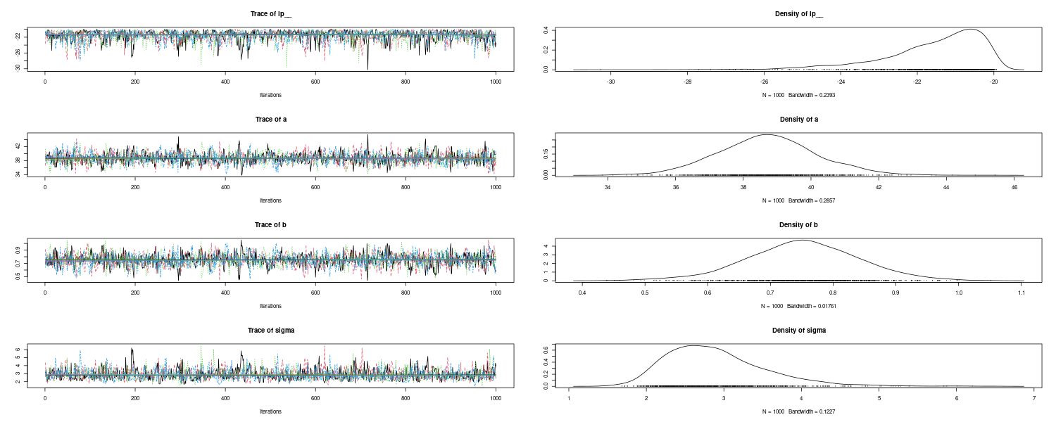

The MCMC sample from the posterior distribution is saved in the fit object (an object of class CmdStanMCMC), and it can be easily drawn by using draws function:

d_ms <- fit$draws(format = "df")
> d_ms
# A draws_df: 1000 iterations, 4 chains, and 4 variables
   lp__  a    b sigma
1   -21 39 0.70   3.0
2   -21 39 0.74   3.4
3   -21 39 0.79   3.1
4   -22 38 0.70   2.3
5   -22 40 0.66   2.0
6   -20 39 0.71   2.3
7   -20 40 0.70   2.8
8   -20 39 0.74   2.3
9   -21 40 0.67   2.5
10  -22 41 0.72   2.6
# ... with 3990 more draws
# ... hidden reserved variables {'.chain', '.iteration', '.draw'}     

ms <- fit$draws(format = "matrix")
> ms
 # A draws_matrix: 1000 iterations, 4 chains, and 4 variables
    variable
draw lp__  a    b sigma
  1   -21 39 0.70   3.0
  2   -21 39 0.74   3.4
  3   -21 39 0.79   3.1
  4   -22 38 0.70   2.3
  5   -22 40 0.66   2.0
  6   -20 39 0.71   2.3
  7   -20 40 0.70   2.8
  8   -20 39 0.74   2.3
  9   -21 40 0.67   2.5
  10  -22 41 0.72   2.6
# ... with 3990 more draws

Adjust the Setings of MCMC

With the default settings for the sample function, the number of chains (chains) is 4, the number of sampling (post-warmup) iterations per chain (iter_sampling) is 1000, the number of warmup iterations per chain (iter_warmup) is 1000. The thinning interval (thin) is 1. The total number of obtained draws are chains * iter_sampling/thin, thus here it is 4*1000/1, which gives 4000.

It is possible to modify these settings and set up initial values:

init_fun <- function(chain_id) {    
  set.seed(chain_id)
  list(
    a = runif(1, 30, 50),
    b = 1,
    sigma = 5
  )
}

fit <- model$sample(
  data = data,
  seed = 123,
  init = init_fun,
  chains = 3,
  iter_warmup = 500,
  iter_sampling = 500,
  thin = 2,
  parallel_chains = 3,
  save_warmup = TRUE
)

When we try a variety of different models, we usually use 300–1000 iterations. But it should be increased once the model is finalized. In general, we implement the model with 2000–10,000 at the final stage, although this also depends on the value of thin. As a reference, if we use MCMC and want to decrease the standard error of posterior mean by one order, based on the central limit theory we know that we need 100 times more draws. Therefore, we need to increase this iter_sampling value when necessary.

For thinning, we usually choose 1 for this argument in Stan, because one advantage of Stan is that there is lower autocorrelation in draws, compared to the other MCMC software such as WinBUGS and JAGS. When some parameter values occasionally have abrupt changes, increasing the value of thin to a larger value (e.g., 5 or 10) can mitigate such changes and reduce autocorrelation, leading to a better convergence.

References

Matsuura K. (2023) Bayesian Statistical Modeling with Stan, R, and Python

Bayesian Statistical Modeling with Stan and R

Contents:

Draw the MCMC Sample