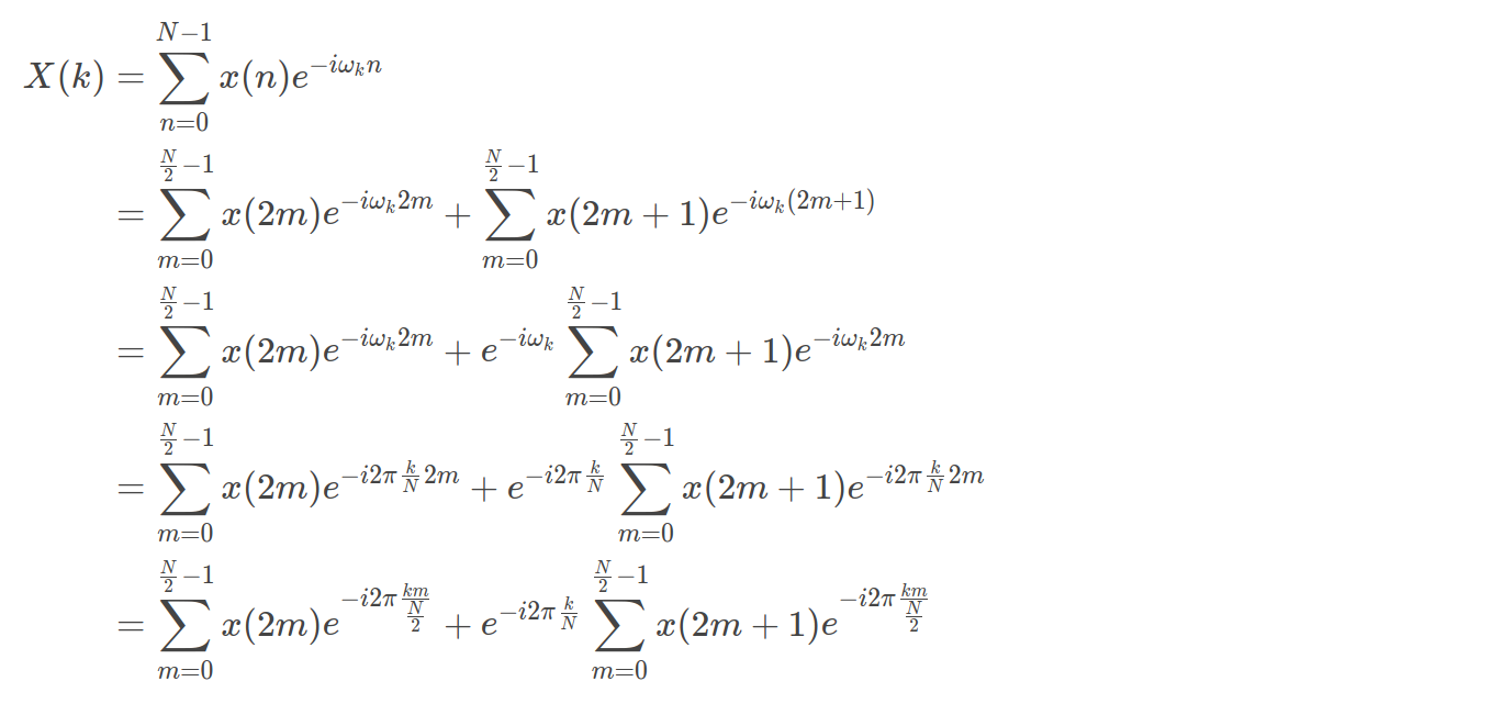
In this post we will talk about Fourier Transform.

Aperiodic Signals

Fourier series assumes that the signal is periodic. But what do we do if the isignal is aperiodic? A trick is to extend the fundamental period from \(T_{0}\) to \(\infty\) when representing it using Fourier series coefficients.

Recall the fourier series coefficients for a continous-time signal:

\[\begin{aligned} C_{k} &= \frac{1}{T_{0}}\int_{\frac{-T_{0}}{2}}^{\frac{T_{0}}{2}}f(t)e^{-i\omega_{0} kt}\ dt \end{aligned}\]

The period as a function of frequency \(\omega_{0}\):

\[\begin{aligned} \omega_{0} &= \frac{2\pi}{T_{0}}\\ \frac{2}{T_{0}} &= \frac{\omega_{0}}{2\pi} \end{aligned}\]

And taking the limit to \(\infty\), \(\omega_{0}\) will be infinitesimally small and represented by \(\Delta \omega\):

\[\begin{aligned} \lim_{T_{0} \to \infty}\frac{2}{T_{0}} &\approx \frac{\Delta \omega}{2\pi} \end{aligned}\]

We re-write \(C_{k}\) equation:

\[\begin{aligned} C_{k} &= \frac{\Delta \omega}{2\pi}\int_{\frac{-T_{0}}{2}}^{\frac{T_{0}}{2}}f(t)e^{-i\omega_{0} kt}\ dt \end{aligned}\]

Inserting this into the fourier series:

\[\begin{aligned} x(t) &= \sum_{k = -\infty}^{\infty}\Big\{ \frac{\Delta \omega}{2\pi}\int_{\frac{-T_{0}}{2}}^{\frac{T_{0}}{2}}f(t)e^{-i\omega_{0} kt}\ dt\Big\}e^{ik\omega_{0}t} \end{aligned}\]

We re-write the equation as:

\[\begin{aligned} x(t) &= \frac{1}{2\pi}\sum_{k = -\infty}^{\infty}\Big\{ \int_{-\infty}^{\infty}f(t)e^{-i\omega_{0} kt}\ dt\Big\}e^{ik\omega t}\ d\omega\\ &= \frac{1}{2\pi}\sum_{k = -\infty}^{\infty}X(\omega)e^{ik\omega t}\ d\omega \end{aligned}\]

Essentially we have broken up the signal into its frequency components as weights and multiplying them by the orthogonal basis function \(e^{ik\omega t}\) and adding them up. Note that if \(X(\omega)\) is symmetric, the imaginary components (\(i sin(\omega)t\)) will cancel out and result in a real signal.

\(X(\omega)\) defined as the Fourier transform:

\[\begin{aligned} X(\omega) &= \int_{-\infty}^{\infty}f(t)e^{-i\omega t}\ dt \end{aligned}\]

And the following is the Inverse Fourier Transform:

\[\begin{aligned} x(t) &= \frac{1}{2\pi}\sum_{k = -\infty}^{\infty}X(\omega)e^{ik\omega t}\ d\omega \end{aligned}\]

We can also write out the Fourier Transform in terms of its magnitude and phase:

\[\begin{aligned} X(\omega) &= |X(\omega)|e^{i \angle X(\omega)} \end{aligned}\]

The whole derivation above is to show that it is possible to do a Fourier Transform on an aperiodic signal.

Delta Function

Dirac defined the delta function as a sum of infinite number of exponentials:

\[\begin{aligned} \delta(t) &= \frac{1}{2\pi}\int_{-\infty}^{\infty}e^{i\omega t}\ d\omega \end{aligned}\]

And in the frequency domain:

\[\begin{aligned} \delta(t) &= \frac{1}{2\pi}\int_{-\infty}^{\infty}e^{i\omega t}\ dt \end{aligned}\]

The general version with time/frequency shift:

\[\begin{aligned} \delta(t - t_{0}) &= \frac{1}{2\pi}\int_{-\infty}^{\infty}e^{i\omega (t - t_{0})}\ d\omega\\[5pt] \delta(\omega - \omega_{0}) &= \frac{1}{2\pi}\int_{-\infty}^{\infty}e^{i(\omega - \omega_{0})t}\ dt \end{aligned}\]

Periodic Signals

A periodic signal can be represented in FSC (Fourier Series Coefficients) form:

\[\begin{aligned} x(t) &= \sum_{k = -\infty}^{\infty}C_{k}e^{i\omega_{0}t} \end{aligned}\]

Taking the fourier transform:

\[\begin{aligned} X(\omega) &= \mathcal{F}\{x(t)\}\\ &= \mathcal{F}\Big\{\sum_{k = -\infty}^{\infty}C_{k}e^{i\omega_{0}t}\Big\}\\ &= \sum_{k = -\infty}^{\infty}C_{k}\mathcal{F}\{e^{i\omega_{0}t}\}\\ \end{aligned}\]

It boils down to taking the fourier transform of an exponential signal:

\[\begin{aligned} e^{i\omega_{0}t} &= \mathrm{cos}(\omega_{0}t) + i \mathrm{sin}(\omega_{0}t)\\ X(e^{i\omega_{0}t}) &= X(\mathrm{cos}(\omega_{0}t)) + i X(\mathrm{sin}(\omega_{0}t))\\ \end{aligned}\]

Fourier transform of a cosine:

\[\begin{aligned} X(\omega) &= \mathcal{F}(\mathrm{cos}(\omega_{0}t))\\ &= \int_{-\infty}^{\infty}\frac{1}{2}(e^{i\omega_{0}t} + e^{-i\omega_{0}t})e^{i\omega t}\ dt\\ &= \int_{-\infty}^{\infty}\frac{1}{2}e^{i(\omega_{0} + \omega_{0})t}\ dt + \int_{-\infty}^{\infty}\frac{1}{2}e^{i(\omega_{0} - \omega_{0})t}\ dt \end{aligned}\]

As discussed in the Delta Function section, we can see that:

\[\begin{aligned} \delta(\omega - \omega_{0}) &= \frac{1}{2\pi}\int_{-\infty}^{\infty}e^{i(\omega - \omega_{0})t}\ dt\\ \pi\delta(\omega - \omega_{0}) &= \frac{1}{2}\int_{-\infty}^{\infty}e^{i(\omega - \omega_{0})t}\ dt\\ \end{aligned}\]

Hence:

\[\begin{aligned} \mathcal{F}\{cos(\omega_{0}t)\} &= \int_{-\infty}^{\infty}\frac{1}{2}e^{i(\omega + \omega_{0})t}\ dt + \int_{-\infty}^{\infty}\frac{1}{2}e^{i(\omega - \omega_{0})t}\ dt\\ &= \pi\delta(\omega + \omega_{0}) + \pi\delta(\omega - \omega_{0}) \end{aligned}\]

Similarly, for sine:

\[\begin{aligned} X(\omega) &= \mathcal{F}\{\mathrm{sin}(\omega_{0}t)\}\\ &= i\pi\delta(\omega + \omega_{0}) - i\pi\delta(\omega - \omega_{0}) \end{aligned}\]

Using the above result:

\[\begin{aligned} X(e^{i\omega_{0}t}) &= X(\mathrm{cos}(\omega_{0}t)) + i X(\mathrm{sin}(\omega_{0}t))\\ &= \pi\delta(\omega+\omega_{0}) + \pi\delta(\omega - \omega_{0}) + i^{2}(\pi\delta(\omega + \omega_{0}) - i^{2}\pi\delta(\omega-\omega_{0}))\\ &= \pi\delta(\omega-\omega_{0}) - i^{2}\pi\delta(\omega - \omega_{0}) + \pi\delta(\omega + \omega_{0}) + i^{2}\pi\delta(\omega + \omega_{0})\\ &= \pi\delta(\omega-\omega_{0}) + \pi\delta(\omega - \omega_{0}) + \pi\delta(\omega + \omega_{0}) - \pi\delta(\omega + \omega_{0})\\ &= 2\pi\delta(\omega - \omega_{0}) \end{aligned}\]

Back to the fourier transform of a periodic signal:

\[\begin{aligned} X(\omega) &= \mathcal{F}\{x(t)\}\\ &= \mathcal{F}\Big\{\sum_{k = -\infty}^{\infty}C_{k}e^{i\omega_{0}t}\Big\}\\ &= \sum_{k = -\infty}^{\infty}C_{k}\mathcal{F}\{e^{i\omega_{0}t}\}\\ &= 2\pi \sum_{k = -\infty}^{\infty}C_{k}\delta(\omega - k\omega_{0}) \end{aligned}\]

This is essentially the same as the discrete fourier series coefficient of the signal but scaled to be \(2\pi\) bigger. This is due to \(X(\omega)\) being periodic with a period of \(2\pi\).

Discrete Fourier Transform

Up till now, what we have been referring to is the Continuous Fourier Transfor:

\[\begin{aligned} X(\omega) &= \int_{-\infty}^{\infty}f(t)e^{-i\omega t}\ dt \end{aligned}\]

For DFT:

\[\begin{aligned} X(k) &= \sum_{n = 0}^{N - 1}x(n)e^{-i\omega_{k} n}\\[5pt] \omega_{k} &= 2\pi \frac{k}{N}\\[5pt] k &= \{0, \cdots, N-1\} \end{aligned}\]

Instead of t, we replaced it with \(n\). And we are dividing \(\omega_{k}\) into \(N\) parts spanning \(2\pi\) interval.

If you look closely at the DFT equation, you could see that it is essentially finding the correlation of the \(N\) sample data against \(N\) equally spaced complex frequencies \(e^{-i\omega_{k} n}\) which are orthogonal basis functions.

For IDFT (Inverse Discrete FT):

\[\begin{aligned} x_{n} &= \frac{1}{N}\sum_{k = 0}^{N-1}X_{k}e^{+i \omega_{k}n}\\[5pt] \omega_{k} &= 2\pi \frac{k}{N}\\[5pt] n &= \{0, \cdots, N-1\} \end{aligned}\]

So \(N\) number of time series data points are transformed to \(N\) frequency points, and the inverse transform will transform \(N\) frequency points back into \(N\) data points.

Note that there are \(N\) multiplications for each \(k\) and there are \(N\) multiplications, resulting in \(N^{2}\) muliplications which grows computationally large for large \(N\). We shall look at Fast Fourier Transform next to cut the computational time to \(N \mathrm{log}(N)\).

Let us take a cosine wave with the following info:

\[\begin{aligned} f &= 1\\ f_{s} &= 16\\ f_{n} &= \frac{16}{2}\\ &= 8 \end{aligned}\]

In other words, the frequency of the cosine curve is 1Hz. Sampling requency \(f_{s}\) is 8Hz (FFT works well with powers of 2) and the Nyquist frequency \(f_{n}\) is 4Hz. This means that the maximum frequency that can be detected is 4Hz. Any higher will result in aliasing and mathematically it cannot detect the difference.

Using R FFT routine to verify the result, we get the following result:

fs <- 8
fn <- fs / 2
f <- 1
omega <- 2 * pi * f
n <- seq(0, 1, length = fs)
xn <- cos(omega * n[1:length(n)])
fft(xn)

> xn
[1]  1.0000000
[2]  0.6234898
[3] -0.2225209
[4] -0.9009689
[5] -0.9009689
[6] -0.2225209
[7]  0.6234898
[8]  1.0000000

> fft(xn)
[1]  0.9999999999999990007993+0.0000000i
[2]  3.8433767734721757669547+1.5919788i
[3] -0.3019377358048381254640-0.3019377i
[4] -0.0414390376673379190464-0.1000427i
[5]  0.0000000000000007771561+0.0000000i
[6] -0.0414390376673376970018+0.1000427i
[7] -0.3019377358048382364863+0.3019377i
[8]  3.8433767734721762110439-1.5919788i       

We can see index 2 has the highest value. Because we start with \(n = 0\), and R starts with index 1, index 2 has \(k = 1\) and index 1 is the DC offset.

\[\begin{aligned} \text{index 1} &= \text{DC Offset}\\ \text{index 2} &= \text{1 Hz}\\ \text{index 3} &= \text{2 Hz}\\ \text{index 4} &= \text{3 Hz}\\ \text{index 5} &= \text{4 Hz}\\ \text{index 5} &= \text{3 Hz}\\ \text{index 5} &= \text{2 Hz}\\ \text{index 5} &= \text{1 Hz} \end{aligned}\]

Anything higher than the Nyquist rate will result in aliasing, so the result is repeated but reflected.

We will do a calculation for index 2:

\[\begin{aligned} \omega_{k = 1} = &2\pi\frac{1}{16}\\ X(k = 1) = &\sum_{n = 0}^{N-1}x(n)e^{-i\omega_{k}n}\\ =\ &1.0000000 \times e^{-i\omega_{1}0} + 0.6234898 \times e^{-i\omega_{1}1} +\\ &-0.2225209 \times e^{-i\omega_{1}2} + -0.9009689 \times e^{-i\omega_{1}3} +\\ &-0.9009689 \times e^{-i\omega_{1}4} + -0.2225209 \times e^{-i\omega_{1}5} +\\ &0.6234898 \times e^{-i\omega_{1}6} + 1.0000000 \times e^{-i\omega_{1}7} \end{aligned}\]

Using R to calculate the value:

omega_k <- 2 * pi * 1/fs
> 1.0000000 * exp(-1i * omega_k * 0) +
  0.6234898 * exp(-1i * omega_k * 1) +
  -0.2225209 * exp(-1i * omega_k * 2) +
  -0.9009689 * exp(-1i * omega_k * 3) +
  -0.9009689 * exp(-1i * omega_k * 4) +
  -0.2225209 * exp(-1i * omega_k * 5) +      
  0.6234898 * exp(-1i * omega_k * 6) +
  1.0000000 * exp(-1i * omega_k * 7)
[1] 3.843377+1.591979i

We can see it agrees with the value we got from FFT.

Fast Fourier Transform (FFT)

FFT is a recursive divide and conquer algorithm that reduces the time complexity of Fourier Transform from \(O(N^{2})\) to \(O\Big(N\mathrm{log}(N)\Big)\). It is termed as one of the most important algorithm of all time. The key idea is there are alot of repeated symmetries in the calculation of \(X(\omega)\), and they only need to be calculated once.

Firstly, let us do the Fourier Transform the long way:

\[\begin{aligned} X(k) &= \sum_{n = 0}^{N - 1}x(n)e^{-i\omega_{k} n}\\ k &= \{0, \cdots, N - 1 \} \end{aligned}\]

res <- c()
N <- length(xn)
for (k in 0:(N - 1)) {
  res2 <- 0
  for(j in 0:(N - 1)) {
    res2 <- res2 + xn[j + 1] * exp(-1i * 2 * pi * k * j / N)       
  }
  res <- c(res, res2)
}
> res
[1]  1.000000e+00+0.000000e+00i  3.843377e+00+1.591979e+00i
[3] -3.019377e-01-3.019377e-01i -4.143904e-02-1.000427e-01i
[5]  8.881784e-16-5.040594e-16i -4.143904e-02+1.000427e-01i
[7] -3.019377e-01+3.019377e-01i  3.843377e+00-1.591979e+00i

Next we divide the series into 2 parts. Even \(2m\) and odd \(2m+1\):

\[\begin{aligned} X(k) &= \sum_{n = 0}^{N - 1}x(n)e^{-i\omega_{k} n}\\ &= \sum_{m = 0}^{\frac{N}{2} - 1}x(2m)e^{-i\omega_{k} 2m} + \sum_{m = 0}^{\frac{N}{2} - 1}x(2m + 1)e^{-i\omega_{k} (2m + 1)}\\ &= \sum_{m = 0}^{\frac{N}{2} - 1}x(2m)e^{-i\omega_{k} 2m} + e^{-i\omega_{k}}\sum_{m = 0}^{\frac{N}{2} - 1}x(2m + 1)e^{-i\omega_{k} 2m}\\ &= \sum_{m = 0}^{\frac{N}{2} - 1}x(2m)e^{-i 2\pi \frac{k}{N} 2m} + e^{-i 2\pi \frac{k}{N}}\sum_{m = 0}^{\frac{N}{2} - 1}x(2m + 1)e^{-i 2\pi \frac{k}{N} 2m}\\ &= \sum_{m = 0}^{\frac{N}{2} - 1}x(2m)e^{-i 2\pi \frac{km}{\frac{N}{2}}} + e^{-i 2\pi \frac{k}{N}}\sum_{m = 0}^{\frac{N}{2} - 1}x(2m + 1)e^{-i 2\pi \frac{km}{\frac{N}{2}}} \end{aligned}\]

In each step, we break the equation into two parts and each part is half the size of the parent. We can then recursively reduce the series by half and end up with only 1 element and:

\[\begin{aligned} x(0)e^{-i\omega_{k}\times 0} &= x(0) \end{aligned}\]

Note that the factor \(e^{i\omega_{k}}\) does not depend on \(m\) and is the same for all \(N - 1\) recursions.

Below is the algorithm implemented in R and using the earlier cosine example:

fft <- function(x, k = 1) {
  n <- length(x)

  if (n == 1) {
    return(x)
  }

  even <- fft3(x[seq(1, n, 2)], k)
  odd <- fft3(x[seq(2, n, 2)], k)
  factor <- exp(-1i * 2 * pi / n * k)    

  result <- even + odd * factor

  result
}

> for (k in 1:length(xn)) {
+   print(fft(xn, k))
+ }
[1] 3.843377+1.591979i
[1] -0.3019377-0.3019377i
[1] -0.041439-0.1000427i
[1] 7.771561e-16-5.040594e-16i
[1] -0.041439+0.1000427i
[1] -0.3019377+0.3019377i
[1] 3.843377-1.591979i
[1] 1+0i

Let us do all \(k\) in one function:

fft <- function(x) {
  n <- length(x)

  if (n == 1) {
    return(x)
  }

  even <- fft(x[seq(1, n, 2)])
  odd <- fft(x[seq(2, n, 2)])
  factor1 <- exp(-1i * 2 * pi / n * seq(0, n / 2 - 1))
  factor2 <- exp(-1i * 2 * pi / n * seq(n / 2, n - 1))

  result <- c(even + factor1 * odd, even + factor2 * odd)

  result
}

> fft(xn)
[1]  1.000000e+00+0.000000e+00i  3.843377e+00+1.591979e+00i
[3] -3.019377e-01-3.019377e-01i -4.143904e-02-1.000427e-01i
[5]  7.771561e-16-6.123234e-17i -4.143904e-02+1.000427e-01i       
[7] -3.019377e-01+3.019377e-01i  3.843377e+00-1.591979e+00i

Note we have 2 factors in the function.

Because we have broken down each even and odd by half, they each would have length \(\frac{N}{2}\). In other words, the even and odd parts are periodic over \(\pm\frac{N}{2}\). We can then reduce that to only one factor (and cut down the amount of work by half).

\[\begin{aligned} X\Big(k + \frac{N}{2}\Big) &= \sum_{m = 0}^{\frac{N}{2} - 1}x(2m)e^{-i\omega_{k + \frac{N}{2}} 2m} + e^{-i\omega_{k + \frac{N}{2}}} \sum_{m = 0}^{\frac{N}{2} - 1}x(2m + 1)e^{-i\omega_{k + \frac{N}{2}} 2m}\\ &= \sum_{m = 0}^{\frac{N}{2} - 1}x(2m)e^{-i\omega_{k} 2m} + e^{-i\omega_{k + \frac{N}{2}}} \sum_{m = 0}^{\frac{N}{2} - 1}x(2m + 1)e^{-i\omega_{k} 2m} \end{aligned}\]

Since:

\[\begin{aligned} e^{-i\omega_{k + \frac{N}{2}}} &= e^{-i\omega_{k} - i\omega_{\frac{N}{2}}}\\ &= e^{-i\omega_{k} - i 2\pi \frac{N}{2N}}\\ &= e^{-i\omega_{k}}e^{- i \pi}\\ &= -1 \times e^{-i\omega_{k}}\\ &= -e^{-i\omega_{k}} \end{aligned}\] \[\begin{aligned} X\Big(k + \frac{N}{2}\Big) &= \sum_{m = 0}^{\frac{N}{2} - 1}x(2m)e^{-i\omega_{k} 2m} + e^{-i\omega_{k + \frac{N}{2}}} \sum_{m = 0}^{\frac{N}{2} - 1}x(2m + 1)e^{-i\omega_{k} 2m}\\ &= \sum_{m = 0}^{\frac{N}{2} - 1}x(2m)e^{-i\omega_{k} 2m} - e^{-i\omega_{k}} \sum_{m = 0}^{\frac{N}{2} - 1}x(2m + 1)e^{-i\omega_{k} 2m} \end{aligned}\]

In summary:

\[\begin{aligned} X(k) &= \sum_{m = 0}^{\frac{N}{2} - 1}x(2m)e^{-i\omega_{k} 2m} + e^{-i\omega_{k}} \sum_{m = 0}^{\frac{N}{2} - 1}x(2m + 1)e^{-i\omega_{k} 2m}\\ X\Big(k + \frac{N}{2}\Big) &= \sum_{m = 0}^{\frac{N}{2} - 1}x(2m)e^{-i\omega_{k} 2m} - e^{-i\omega_{k}} \sum_{m = 0}^{\frac{N}{2} - 1}x(2m + 1)e^{-i\omega_{k} 2m} \end{aligned}\]

We can simplify the above code using the above equation as follows:

fft <- function(x) {
  n <- length(x)

  if (n == 1) {
    return(x)
  }

  even <- fft2(x[seq(1, n, 2)])
  odd <- fft2(x[seq(2, n, 2)])

  factor <- exp(-1i * 2 * pi / n * seq(0, n / 2 - 1))

  result <- c(even + factor * odd, even - factor * odd)

  result
}
> fft(xn)
[1]  1.000000e+00+0.000000e+00i  3.843377e+00+1.591979e+00i
[3] -3.019377e-01-3.019377e-01i -4.143904e-02-1.000427e-01i      
[5]  7.771561e-16+0.000000e+00i -4.143904e-02+1.000427e-01i
[7] -3.019377e-01+3.019377e-01i  3.843377e+00-1.591979e+00i

Note that the above algorithm assumes the number of elements is a power of 2. More work (like padding or other ways) are needed to support non-power of 2.

Inverse Fourier Transform

To recap:

\[\begin{aligned} x_{n} &= \frac{1}{N}\sum_{k = 0}^{N-1}X_{k}e^{+i \omega_{k}n}\\[5pt] \omega_{k} &= 2\pi \frac{k}{N}\\[5pt] n &= \{0, \cdots, N-1\} \end{aligned}\]

Using the same example as before:

> fft(xn)
[1]  0.9999999999999990007993+0.0000000i  3.8433767734721757669547+1.5919788i
[3] -0.3019377358048381254640-0.3019377i -0.0414390376673379190464-0.1000427i
[5]  0.0000000000000007771561+0.0000000i -0.0414390376673376970018+0.1000427i
[7] -0.3019377358048382364863+0.3019377i  3.8433767734721762110439-1.5919788i       

Firstly, let us do the long calculation that has \(O(n^{2})\) time complexity:

fs <- 8
fn <- fs / 2
f <- 1
omega <- 2 * pi * f
n <- seq(0, 1, length = fs)
xn <- cos(omega * n[1:length(n)])
freqs <- fft(xn)

N <- length(xn)
xn2 <- rep(0, N)
for (n in 1:N) {
  for (k in 1:N) {
    xn2[n] <- xn2[n] + freqs[k] * exp(1i * 2 * pi * (k - 1) / N * (n - 1))
  }
}
> Re(xn2 / N)
[1]  1.0000000  0.6234898 -0.2225209 -0.9009689 -0.9009689 -0.2225209  0.6234898  1.0000000
> xn
[1]  1.0000000  0.6234898 -0.2225209 -0.9009689 -0.9009689 -0.2225209  0.6234898  1.0000000       

We can see that the result match with each other. Next we employ inverse FFT. FFT and IFFT have similar form, so the computation for FFT can be easily generalized to IFFT:

gsignal::ifft(freqs)
[1]  1.0000000  0.6234898 -0.2225209 -0.9009689 -0.9009689 -0.2225209  0.6234898  1.0000000       

Fourier Series vs Fourier Transform

Let us see the representation from both fourier series and fourier transform on \(x(t)\):

\[\begin{aligned} x(t) &= \sum_{k = -\infty}^{\infty}C_{k}e^{ik\omega_{0}t}\\ x(t) &= \frac{1}{2\pi}\int_{-\infty}^{\infty}X(\omega)e^{ik\omega t}\ d\omega\\ x_{n} &= \frac{1}{N}\sum_{k = 0}^{N-1}X_{k}e^{+i \omega_{k}n} \end{aligned}\]

The main reason why we do a Fourier tranform rather than FSC is because Fourier Transform can be used for both aperiodic and periodic signals.

See Also

Fourier Series

References

The Intuitive Guide to Fourier Analysis and Spectral Estimation: with Matlab

Iain Explains Signals, Systems, and Digital Comms (YouTube)

Python Numerical Methods

An Introduction and Analysis of the Fast Fourier Transform (Thao Nguyen)